05. Total vs primary/secondary field

We usually use emg3d for total field computations. However, we can also use it in a primary-secondary field formulation, where we compute the primary field with a (semi-)analytical solution.

In this example we use emg3d to compute

• Total field

• Primary field

• Secondary field

and compare the total field to the primary+secondary field.

The primary-field computation could be replaced by a 1D modeller such as empymod. You can play around with the required computation-domain: Using a primary-secondary formulation makes it possible to restrict the required computation domain for the scatterer a lot, therefore speeding up the computation. However, we do not dive into that in this example.

Background

The total field is given by

(1)\[s \mu \sigma \mathbf{\hat{E}} + \nabla \times \nabla \times \mathbf{\hat{E}} = -s\mu\mathbf{\hat{J}}_s .\]

We can split it up into a primary field \(\mathbf{\hat{E}}^p\) and a secondary field \(\mathbf{\hat{E}}^s\),

(2)\[\mathbf{\hat{E}} = \mathbf{\hat{E}}^p + \mathbf{\hat{E}}^s,\]

where we also have to split our conductivity model into

(3)\[\sigma = \sigma^p + \Delta\sigma.\]

The primary field could be just the direct field, or the direct field plus the air layer, or an entire 1D background, something that can be computed (semi-)analytically. The secondary field is everything that is not included in the primary field.

The primary field is then given by

(4)\[s \mu \sigma^p \mathbf{\hat{E}}^p + \nabla \times \nabla \times \mathbf{\hat{E}}^p = -s\mu\mathbf{\hat{J}}_s ,\]

and the secondary field can be computed using the primary field as source,

(5)\[s \mu \sigma \mathbf{\hat{E}}^s + \nabla \times \nabla \times \mathbf{\hat{E}}^s = -s\mu\Delta\sigma\mathbf{\hat{E}}^p .\]

import emg3d
import numpy as np
import matplotlib.pyplot as plt
from matplotlib.colors import LogNorm
plt.style.use('bmh')

Survey

src = [0, 0, -950, 0, 0]    # x-dir. source at the origin, 50 m above seafloor
off = np.arange(5, 81)*100  # Offsets
rec = [off, off*0, -1000]   # In-line receivers on the seafloor
res = [1e10, 0.3, 1]        # 1D resistivities (Ohm.m): [air, water, backgr.]
freq = 1.0                  # Frequency (Hz)

source = emg3d.TxElectricDipole(src)

Mesh

We create quite a coarse grid (100 m minimum cell width), to have reasonable fast computation times.

Also note that the mesh here includes a large boundary because of the air layer. If you use a semi-analytical solution for the 1D background you could restrict that domain a lot.

grid = emg3d.construct_mesh(
        frequency=freq,
        properties=[res[1], 100, res[2], 100],
        center=(src[0], src[1], -1000),
        min_width_limits=(100, 100, 100),
        domain=([-100, 8100], [-500, 500], [-2500, 0]),
        center_on_edge=False,
)

grid

TensorMesh			245,760 cells
		MESH EXTENT		CELL WIDTH		FACTOR
dir	nC	min	max	min	max	max
x	128	-33,640.98	48,527.04	100.00	6,886.06	1.20
y	40	-32,849.73	45,222.36	100.00	12,372.63	1.38
z	48	-6,940.24	32,349.73	100.00	8,973.55	1.38

Create model

# Layered_background
res_x = np.ones(grid.n_cells)*res[0]            # Air resistivity
res_x[grid.cell_centers[:, 2] < 0] = res[1]      # Water resistivity
res_x[grid.cell_centers[:, 2] < -1000] = res[2]  # Background resistivity

# Background model
model_pf = emg3d.Model(grid, property_x=res_x.copy(), mapping='Resistivity')

# Include the target
xx = (grid.cell_centers[:, 0] >= 0) & (grid.cell_centers[:, 0] <= 6000)
yy = abs(grid.cell_centers[:, 1]) <= 500
zz = (grid.cell_centers[:, 2] > -2500)*(grid.cell_centers[:, 2] < -2000)

res_x[xx*yy*zz] = 100.  # Target resistivity

# Create target model
model = emg3d.Model(grid, property_x=res_x, mapping='Resistivity')

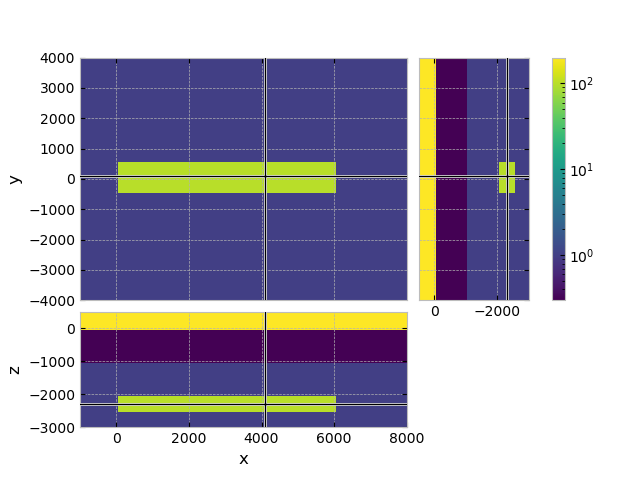
# Plot a slice
grid.plot_3d_slicer(
        model.property_x, zslice=-2250,
        xlim=(-1000, 8000), ylim=(-4000, 4000), zlim=(-3000, 500),
        pcolor_opts={'norm': LogNorm(vmin=0.3, vmax=200)}
)

Compute total field with emg3d

em3_tf = emg3d.solve_source(model, source, freq, verb=1)

:: emg3d :: 7.2e-07; 1(4); 0:00:14; CONVERGED

Compute primary field (1D background) with emg3d

Here we use emg3d to compute the primary field. This could be replaced by a (semi-)analytical solution.

em3_pf = emg3d.solve_source(model_pf, source, freq, verb=1)

:: emg3d :: 7.0e-07; 1(4); 0:00:15; CONVERGED

Compute secondary field (scatterer) with emg3d

Define the secondary source

# Get the difference of conductivity as volume-average values
diff = 1/model.property_x-1/model_pf.property_x
dsigma = grid.cell_volumes.reshape(grid.shape_cells, order='F')*diff

# Here we use the primary field computed with emg3d. This could be done
# with a 1D modeller such as empymod instead.
sfield_sf = em3_pf.copy()

# Average delta sigma to the corresponding edges
sfield_sf.fx[:, 1:-1, 1:-1] *= 0.25*(dsigma[:, :-1, :-1] + dsigma[:, 1:, :-1] +
                                     dsigma[:, :-1, 1:] + dsigma[:, 1:, 1:])
sfield_sf.fy[1:-1, :, 1:-1] *= 0.25*(dsigma[:-1, :, :-1] + dsigma[1:, :, :-1] +
                                     dsigma[:-1, :, 1:] + dsigma[1:, :, 1:])
sfield_sf.fz[1:-1, 1:-1, :] *= 0.25*(dsigma[:-1, :-1, :] + dsigma[1:, :-1, :] +
                                     dsigma[:-1, 1:, :] + dsigma[1:, 1:, :])

# Create field instance -iwu dsigma E
sfield_sf = emg3d.Field(
        sfield_sf.grid, -sfield_sf.field*sfield_sf.smu0, frequency=freq)

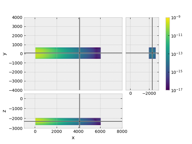
Plot the secondary source

Our secondary source is the entire target, the scatterer. Here we look at the \(E_x\) secondary source field. But note that the secondary source has all three components \(E_x\), \(E_y\), and \(E_z\), even though our primary source was purely \(x\)-directed. (Change fx to fy or fz in the command below, and simultaneously Ex to Ey or Ez, to show the other source fields.)

grid.plot_3d_slicer(
        sfield_sf.fx.ravel('F'), view='abs', v_type='Ex', zslice=-2250,
        xlim=(-1000, 8000), ylim=(-4000, 4000), zlim=(-3000, 500),
        pcolor_opts={'norm': LogNorm(vmin=1e-17, vmax=1e-9)}
)

Compute the secondary source

em3_sf = emg3d.solve(model, sfield_sf, verb=1)

:: emg3d :: 7.7e-07; 2(7); 0:00:25; CONVERGED

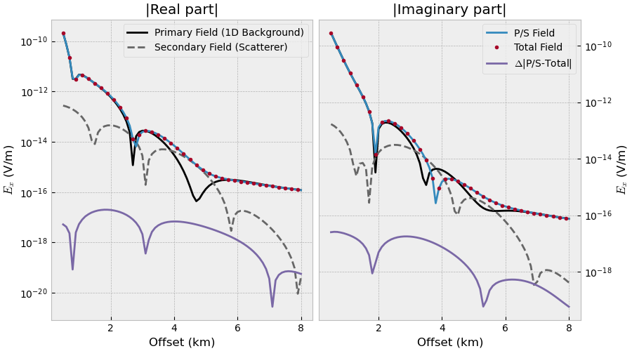
Plot result

# E = E^p + E^s
em3_ps = em3_pf.copy()
em3_ps.field += em3_sf.field

# Get the responses at receiver locations
rectuple = (rec[0], rec[1], rec[2], 0, 0)
em3_pf_rec = em3_pf.get_receiver(rectuple)
em3_tf_rec = em3_tf.get_receiver(rectuple)
em3_sf_rec = em3_sf.get_receiver(rectuple)
em3_ps_rec = em3_ps.get_receiver(rectuple)

fig, (ax1, ax2) = plt.subplots(1, 2, figsize=(9, 5), sharex=True)

ax1.set_title('|Real part|')
ax1.plot(off/1e3, abs(em3_pf_rec.real), 'k',
         label='Primary Field (1D Background)')
ax1.plot(off/1e3, abs(em3_sf_rec.real), '.4', ls='--',
         label='Secondary Field (Scatterer)')
ax1.plot(off/1e3, abs(em3_ps_rec.real))
ax1.plot(off[::2]/1e3, abs(em3_tf_rec[::2].real), '.')
ax1.plot(off/1e3, abs(em3_ps_rec.real-em3_tf_rec.real))
ax1.set_xlabel('Offset (km)')
ax1.set_ylabel('$E_x$ (V/m)')
ax1.set_yscale('log')
ax1.legend()

ax2.set_title('|Imaginary part|')
ax2.plot(off/1e3, abs(em3_pf_rec.imag), 'k')
ax2.plot(off/1e3, abs(em3_sf_rec.imag), '.4', ls='--')
ax2.plot(off/1e3, abs(em3_ps_rec.imag), label='P/S Field')
ax2.plot(off[::2]/1e3, abs(em3_tf_rec[::2].imag), '.', label='Total Field')
ax2.plot(off/1e3, abs(em3_ps_rec.imag-em3_tf_rec.imag),
         label=r'$\Delta$|P/S-Total|')
ax2.set_xlabel('Offset (km)')
ax2.set_ylabel('$E_x$ (V/m)')
ax2.set_yscale('log')
ax2.yaxis.tick_right()
ax2.yaxis.set_label_position("right")
plt.legend()

fig.tight_layout()
fig.show()

emg3d.Report()

Wed Aug 31 21:32:35 2022 CEST
OS	Linux	CPU(s)	4	Machine	x86_64
Architecture	64bit	RAM	15.5 GiB	Environment	Python
File system	ext4
Python 3.9.12 | packaged by conda-forge | (main, Mar 24 2022, 23:22:55) [GCC 10.3.0]
numpy	1.22.4	scipy	1.9.0	numba	0.55.2
emg3d	1.8.0	empymod	2.2.0	xarray	2022.6.0
discretize	0.8.2	h5py	3.7.0	matplotlib	3.4.3
tqdm	4.64.0	IPython	8.4.0
Intel(R) oneAPI Math Kernel Library Version 2022.0-Product Build 20211112 for Intel(R) 64 architecture applications

Estimated memory usage: 236 MB