Note
Go to the end to download the full example code.
SEG-EAGE 3D Salt Model#
[Muld07] presented electromagnetic responses for a resistivity model which he derived from the seismic velocities of the SEG/EAGE salt model [AmBK97].
Here we reproduce and store this resistivity model, and compute electromagnetic responses for it.
Velocity-to-resistivity transform#
Quoting here the description of the velocity-to-resistivity transform used by [Muld07]:
«The SEG/EAGE salt model (Aminzadeh et al. 1997), originally designed for seismic simulations, served as a template for a realistic subsurface model. Its dimensions are 13500 by 13480 by 4680 m. The seismic velocities of the model were replaced by resistivity values. The water velocity of 1.5 km/s was replaced by a resistivity of 0.3 Ohm m. Velocities above 4 km/s, indicative of salt, were replaced by 30 Ohm m. Basement, beyond 3660 m depth, was set to 0.002 Ohm m. The resistivity of the sediments was determined by \((v/1700)^{3.88}\) Ohm m, with the velocity v in m/s (Meju et al. 2003). For air, the resistivity was set to \(10^8\) Ohm m.»
Equation 1 of [MeGM03], is given by
where \(\rho\) is resistivity, \(V_P\) is P-wave velocity, and for \(m\) and \(c\) 3.88 and -11 were used, respectively.
The velocity-to-resistivity transform uses therefore a Faust model ([Faus53]) with some additional constraints for water, salt, and basement.
Note
The SEG/EAGE Salt Model is licensed under the CC-BY-4.0.
import os
import pooch
import emg3d
import numpy as np
import matplotlib.pyplot as plt
from matplotlib.colors import LogNorm
plt.style.use('bmh')


# Adjust this path to a folder of your choice.
data_path = os.path.join('..', 'download', '')
Fetch the model#
Retrieve and load the pre-computed resistivity model.
fname = "SEG-EAGE-Salt-Model.h5"
pooch.retrieve(
    'https://raw.github.com/emsig/data/2021-05-21/emg3d/models/'+fname,
    '6ee10663de588d445332ba7cc1c0dc3d6f9c50d1965f797425cebc64f9c71de6',
    fname=fname,
    path=data_path,
)
fmodel = emg3d.load(data_path + fname)['model']
fgrid = fmodel.grid
Data loaded from «/home/dtr/Codes/emsig/emg3d-gallery/examples/download/SEG-EAGE-Salt-Model.h5»
[emg3d v1.0.0rc3.dev5+g0cd9e09 (format 1.0) on 2021-05-21T13:15:50.617756].
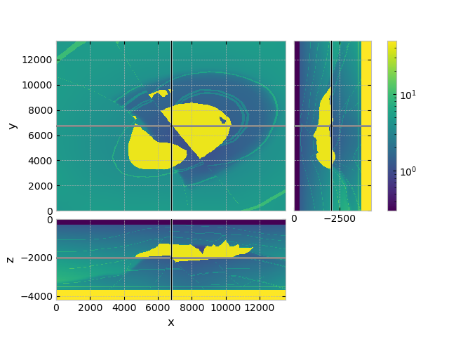
QC resistivity model#
# Limit colour-range to [0.3, 50] Ohm.m
# (affects only the basement and air, improves resolution in the sediments).
vmin, vmax = 0.3, 50

fgrid.plot_3d_slicer(
        fmodel.property_x,
        zslice=-2000,
        pcolor_opts={'norm': LogNorm(vmin=vmin, vmax=vmax)}
)
Compute some example CSEM data with it#
Survey parameters#
# Create a source instance
source = emg3d.TxElectricDipole(
        coordinates=[6400, 6600, 6500, 6500, -50, -50],
        strength=1/200.  # Normalize for length.
)

# Frequency (Hz)
frequency = 1.0
Initialize computation mesh#
grid = emg3d.construct_mesh(
    frequency=frequency,
    properties=[0.3, 1, 2, 15],
    center=(6500, 6500, -50),
    seasurface=0,
    domain=([0, 13500], [0, 13500], None),
    vector=(None, None, np.array([-100, -80, -60, -40, -20, 0])),
    min_width_limits=([5, 100], [5, 100], [5, 20]),
    min_width_pps=5,
    stretching=[1.03, 1.05],
    lambda_from_center=True,
    center_on_edge=True,
)
grid
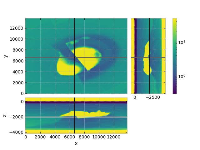
Put the salt model onto the modelling mesh#
# Interpolate full model from full grid to grid
model = fmodel.interpolate_to_grid(grid)

grid.plot_3d_slicer(
        model.property_x,
        zslice=-2000,
        zlim=(-4180, 500),
        pcolor_opts={'norm': LogNorm(vmin=vmin, vmax=vmax)}
)
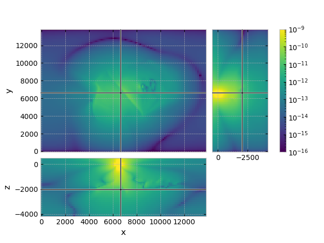
Solve the system#
:: emg3d :: 4.8e-07; 5(10); 0:00:42; CONVERGED
grid.plot_3d_slicer(
    efield.fx.ravel('F'),
    zslice=-2000,
    zlim=(-4180, 500),
    view='abs',
    v_type='Ex',
    pcolor_opts={'norm': LogNorm(vmin=1e-16, vmax=1e-9)}
)
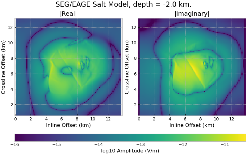
# Interpolate for a "more detailed" image
x = grid.cell_centers_x
y = grid.cell_centers_y
rx = np.repeat([x, ], np.size(x), axis=0)
ry = rx.transpose()
rz = -2000
data = efield.get_receiver((rx, ry, rz, 0, 0))

# Colour limits
vmin, vmax = -16, -10.5

# Create a figure
fig, (ax1, ax2) = plt.subplots(
        1, 2, figsize=(8, 5), sharex=True, constrained_layout=True)

titles = [r'|Real|', r'|Imaginary|']


def log10abs(inp):
    """Log10 of absolute values, avoiding zero-division."""
    tiny = np.finfo(float).tiny
    return np.log10(np.where(abs(inp) < tiny, tiny, abs(inp)))


dat = [log10abs(data.real), log10abs(data.imag)]

for i, ax in enumerate([ax1, ax2]):
    ax.set_title(titles[i])
    cs = ax.pcolormesh(x/1000, x/1000, dat[i], vmin=vmin, vmax=vmax,
                       linewidth=0, rasterized=True, shading='nearest')
    ax.set_xlim([min(x)/1000, max(x)/1000])
    ax.axis('equal')
    ax.set_xlabel('Inline Offset (km)')
    ax.set_ylabel('Crossline Offset (km)')

# Plot colorbar
cb = plt.colorbar(cs, ax=[ax1, ax2], orientation='horizontal', aspect=30)
cb.set_label("log10 Amplitude (V/m)")

# Title
fig.suptitle(f"SEG/EAGE Salt Model, depth = {rz/1e3} km.", fontsize=16)
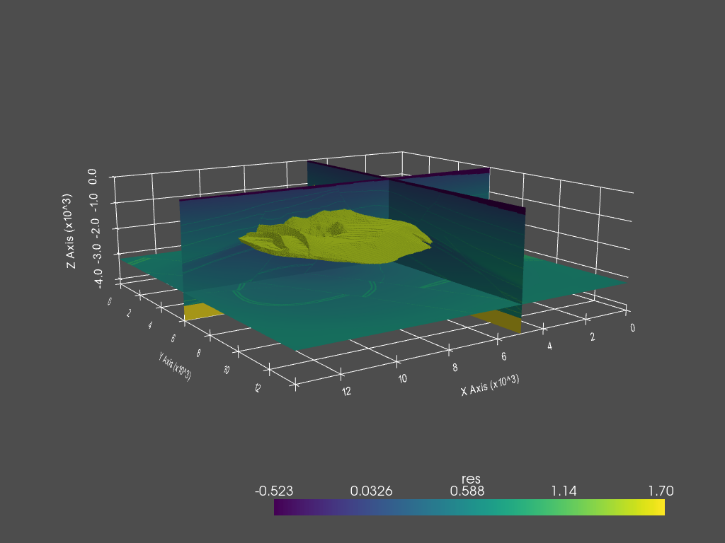
QC resistivity model with PyVista#
Note
The following cell is about how to plot the model in 3D using PyVista,
for which you have to install pyvista.
The code example was created on 2021-05-21 with pyvista=0.30.1.
import pyvista

dataset = fgrid.to_vtk({'res': np.log10(fmodel.property_x.ravel('F'))})

# Create the rendering scene and add a grid axes
p = pyvista.Plotter(notebook=True)
p.show_grid(location='outer')

dparams = {'rng': np.log10([vmin, vmax]), 'show_edges': False}
# Add spatially referenced data to the scene
xyz = (5000, 6000, -3200)
p.add_mesh(dataset.slice('x', xyz), name='x-slice', **dparams)
p.add_mesh(dataset.slice('y', xyz), name='y-slice', **dparams)
p.add_mesh(dataset.slice('z', xyz), name='z-slice', **dparams)

# Get the salt body
p.add_mesh(dataset.threshold([1.47, 1.48]), name='vol', **dparams)

# Show the scene!
p.camera_position = [
    (27000, 37000, 5800), (6600, 6600, -3300), (0, 0, 1)
]
p.show()
Reproduce the resistivity model#
Note
The last cell as about how to reproduce the resistivity model. For this you have to download the SEG/EAGE salt model, as explained further down.
The code example and the SEG-EAGE-Salt-Model.h5-file used in the
gallery were created on 2021-05-21.
To reduce runtime and dependencies of the gallery build we use a pre-computed resistivity model, which was generated with the code provided below.
In order to reproduce it yourself you have to download the data from the
SEG-website or via this
direct link.
The zip-file is 513.1 MB big. Unzip the archive, and place the file
Salt_Model_3D/3-D_Salt_Model/VEL_GRIDS/SALTF.ZIP (20.0 MB) in the same
directory as the notebook.
The following cell loads takes this SALTF.ZIP, carries out the
velocity-to-resistivity transform, and stores the resistivity model for later
use.
import emg3d
import zipfile
import numpy as np

# Dimension of seismic velocities
nx, ny, nz = 676, 676, 210

# Create a discretize-mesh of the correct dimension
# (nz: +1, for air)
fgrid = emg3d.TensorMesh(
    [np.ones(nx)*20., np.ones(ny)*20., np.ones(nz+1)*20.],
    origin=(0, 0, -210*20))
res = np.zeros(fgrid.shape_cells, order='F')

# Load data
zipfile.ZipFile('SALTF.ZIP', 'r').extract('Saltf@@')
with open('Saltf@@', 'r') as file:
    v = np.fromfile(file, dtype=np.dtype('float32').newbyteorder('>'))
    res[:, :, 1:] = v.reshape((nx, ny, nz), order='F')

# Velocity to resistivity transform for whole cube
res = (res/1700)**3.88  # Sediment resistivity = 1

# Overwrite basement resistivity from 3660 m onwards
res[:, :, np.arange(fgrid.shape_cells[2])*20 > 3680] = 500.

# Set sea-water to 0.3
res[:, :, :16][res[:, :, :16] <= 1500] = 0.3
# Ensure at least top layer is water
res[:, :, 1] = 0.3

# Fix salt resistivity
res[res == 4482] = 30.

# Set air resistivity
res[:, :, 0] = 1e8

# THE SEG/EAGE salt-model uses positive z downwards; discretize positive
# upwards. Hence for res, we use np.flip(res, 2) to flip the z-direction
res = np.flip(res, 2)

# Create the resistivity model
model = emg3d.Model(fgrid, property_x=res)

# Store the resistivity model
emg3d.save("SEG-EAGE-Salt-Model.h5", model=model)
Total running time of the script: (0 minutes 48.795 seconds)
Estimated memory usage: 3606 MB