Note
Go to the end to download the full example code.
09. Transient CSEM#
The computation of emg3d happens in the frequency domain (or Laplace
domain), each frequency requires a new computation. Using (inverse) Fourier
transforms, we can also compute time-domain (transient) CSEM data with
emg3d. This is not (yet) implemented in easy, user-friendly functions. It
does require quite some input and knowledge from the user, particularly with
regards to the gridding.
A good starting point to model time-domain data with emg3d is [WeMS21].
You can find the paper and all the notebooks in the repo
emsig/article-TDEM .
The following is a simple example from the above article, the time-domain modelling of a fullspace. It based on the first example (Figures 3-4) of [MuWS08].
Interactive frequency selection#
The most important factor in fast time-domain computation is the frequency selection. You can find an interactive GUI for this in the repo emsig/frequency-selection .
A screenshot of the GUI for the interactive frequency selection is shown in the following figure:
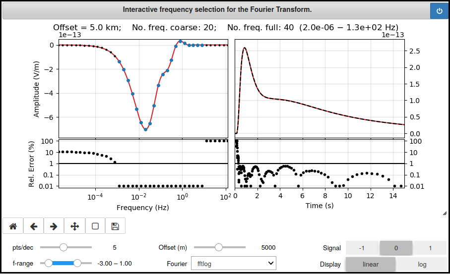
The GUI uses the 1D modeller empymod for a layered model, and internally
the Fourier class of the 3D modeller emg3d. The following parameters
can be specified interactively:
points per decade
frequency range (min/max)
offset
Fourier transform (FFTLog or DLF with different filters)
signal (impulse or switch-on/-off)
Other parameters have to be specified fix when initiating the widget.
import emg3d
import empymod
import numpy as np
import matplotlib.pyplot as plt
plt.style.use('bmh')
Model and Survey#
Model#
Homogeneous fullspace of 1 Ohm.m.
Survey#
Source at origin.
Receiver at an inline-offset of 900 m.
Both source and receiver are x-directed electric dipoles.
src_coo = [0, 0, 0, 0, 0]
source = emg3d.TxElectricDipole(src_coo)
rec_coo = [900, 0, 0, 0, 0]
resistivity = 1                  # Fullspace resistivity
depth = []
Fourier Transforms parameters#
We only compute frequencies \(0.05 < f < 21\) Hz, which yields enough precision for our purpose.
This means, instead of 30 frequencies from 0.0002 - 126.4 Hz, we only need 14 frequencies from 0.05 - 20.0 Hz.
# Define desired times.
time = np.logspace(-2, 1, 201)

# Initiate a Fourier instance
Fourier = emg3d.Fourier(
    time=time,
    fmin=0.05,
    fmax=21,
    ft='fftlog',  # Fourier transform to use
    ftarg={'pts_per_dec': 5, 'add_dec': [-2, 1], 'q': 0},
)

# Dense frequencies for comparison reasons
freq_dense = np.logspace(
    np.log10(Fourier.freq_required.min()),
    np.log10(Fourier.freq_required.max()),
    301,
)
time        [s] :  0.01 - 10 : 201  [min-max; #]
signal          :  0
Fourier         :  FFTLog
  > pts_per_dec :  5
  > add_dec     :  [-2.  1.]
  > q           :  0.0
Req. freq  [Hz] :  0.000200364 - 126.421 : 30  [min-max; #]
Calc. freq [Hz] :  0.0503292 - 20.0364 : 14  [min-max; #]
Frequency-domain computation#
# Automatic gridding settings.
grid_opts = {
    'center': src_coo[:3],           # Source location
    'domain': [[-200, 1100], [-50, 50], [-50, 50]],
    'properties': resistivity,       # Fullspace resistivity.
    'min_width_limits': [20., 40.],  # Restrict cell width within survey domain
    'min_width_pps': 12,             # Many points to have small min cell width
    'stretching': [1, 1.3],          # <alpha improves result, slows down comp
    'lambda_from_center': True,      # 2 lambda from src to boundary and back
    'center_on_edge': False,
}

# Initiate data array and log dict.
data = np.zeros(Fourier.freq_compute.size, dtype=complex)
log = {}

# Loop over frequencies, going from high to low.
for fi, freq in enumerate(Fourier.freq_compute[::-1]):
    print(f"  {fi+1:2}/{Fourier.freq_compute.size} :: {freq:10.6f} Hz",
          end='\r')

    # Construct mesh and model.
    grid = emg3d.meshes.construct_mesh(frequency=freq, **grid_opts)
    model = emg3d.Model(grid, property_x=resistivity)

    # Interpolate the starting electric field from the last one (can speed-up
    # the computation).
    if fi == 0:
        efield = emg3d.Field(grid, frequency=freq)
    else:
        efield = efield.interpolate_to_grid(grid)

    # Solve the system.
    info = emg3d.solve_source(
        model, source, freq, efield=efield, verb=0,
        return_info=True, tol=1e-6/freq,  # f-dep. tolerance
    )

    # Store response at receivers.
    data[-fi-1] = efield.get_receiver(rec_coo)

    # Store some info in the log.
    log[str(int(freq*1e6))] = {
        'freq': freq,
        'nC': grid.nC,
        'stretching': max(
            np.r_[grid.h[0][1:]/grid.h[0][:-1], grid.h[0][:-1]/grid.h[0][1:],
                  grid.h[1][1:]/grid.h[1][:-1], grid.h[1][:-1]/grid.h[1][1:],
                  grid.h[2][1:]/grid.h[2][:-1], grid.h[2][:-1]/grid.h[2][1:]]
        ),
        'dminmax': [np.min(np.r_[grid.h[0], grid.h[1], grid.h[2]]),
                    np.max(np.r_[grid.h[0], grid.h[1], grid.h[2]])],
        'info': info,
    }

    # Store the grid for the interpolation.
    old_grid = grid
   1/14 ::  20.036420 Hz
/home/dtr/Codes/emsig/emg3d-gallery/examples/tutorials/timedomain.py:153: DeprecationWarning: Conversion of an array with ndim > 0 to a scalar is deprecated, and will error in future. Ensure you extract a single element from your array before performing this operation. (Deprecated NumPy 1.25.)
  data[-fi-1] = efield.get_receiver(rec_coo)
   2/14 ::  12.642126 Hz
   3/14 ::   7.976643 Hz
   4/14 ::   5.032921 Hz
   5/14 ::   3.175559 Hz
   6/14 ::   2.003642 Hz
   7/14 ::   1.264213 Hz
   8/14 ::   0.797664 Hz
   9/14 ::   0.503292 Hz
  10/14 ::   0.317556 Hz
  11/14 ::   0.200364 Hz
  12/14 ::   0.126421 Hz
  13/14 ::   0.079766 Hz
  14/14 ::   0.050329 Hz
runtime = 0
for freq in Fourier.freq_compute[::-1]:
    value = log[str(int(freq*1e6))]
    print(f"  {value['freq']:7.3f} Hz: {value['info']['it_mg']:2g}/"
          f"{value['info']['it_ssl']:g} it; "
          f"{value['info']['time']:4.0f} s; "
          f"max_a: {value['stretching']:.2f}; "
          f"nC: {value['nC']:8,.0f}; "
          f"h: {value['dminmax'][0]:5.0f} / {value['dminmax'][1]:7.0f}")
    runtime += value['info']['time']

print(f"\n                **** TOTAL RUNTIME :: {runtime // 60:.0f} min "
      f"{runtime % 60:.1f} s ****\n")
20.036 Hz:  6/1 it;    2 s; max_a: 1.26; nC:   46,080; h:    20 /     208
12.642 Hz:  6/1 it;    4 s; max_a: 1.16; nC:   98,304; h:    20 /     167
 7.977 Hz:  6/1 it;    4 s; max_a: 1.19; nC:   98,304; h:    20 /     239
 5.033 Hz:  6/1 it;    4 s; max_a: 1.22; nC:   98,304; h:    20 /     340
 3.176 Hz:  6/1 it;    3 s; max_a: 1.25; nC:   81,920; h:    24 /     443
 2.004 Hz:  6/1 it;    3 s; max_a: 1.23; nC:   81,920; h:    30 /     558
 1.264 Hz:  6/1 it;    2 s; max_a: 1.21; nC:   65,536; h:    37 /     620
 0.798 Hz:  6/1 it;    2 s; max_a: 1.23; nC:   65,536; h:    40 /     863
 0.503 Hz:  6/1 it;    2 s; max_a: 1.25; nC:   65,536; h:    40 /    1200
 0.318 Hz:  6/1 it;    2 s; max_a: 1.28; nC:   65,536; h:    40 /    1658
 0.200 Hz:  6/1 it;    4 s; max_a: 1.27; nC:  102,400; h:    40 /    1825
 0.126 Hz:  6/1 it;    4 s; max_a: 1.30; nC:  102,400; h:    40 /    2564
 0.080 Hz:  6/1 it;    5 s; max_a: 1.25; nC:  128,000; h:    40 /    2974
 0.050 Hz:  6/1 it;    5 s; max_a: 1.27; nC:  128,000; h:    40 /    3909

             **** TOTAL RUNTIME :: 0 min 45.8 s ****
Frequency domain#
Compute analytical result and interpolate missing responses
data_int = Fourier.interpolate(data)

# Compute analytical result using empymod
epm_req = empymod.bipole(src_coo, rec_coo, depth, resistivity,
                         Fourier.freq_required, verb=1)
epm_dense = empymod.bipole(src_coo, rec_coo, depth, resistivity,
                           freq_dense, verb=1)

# Compute error
err = np.clip(100*abs((data_int.imag-epm_req.imag)/epm_req.imag), 0.1, 100)
Time domain#
Do the transform and compute analytical result.
# Compute corresponding time-domain signal.
data_time = Fourier.freq2time(data, rec_coo[0])

# Analytical result
epm_time = empymod.analytical(src_coo[:3], rec_coo[:3], resistivity, time,
                              solution='dfs', signal=0, verb=1)

# Relative error and peak error
err_egd = 100*abs((data_time-epm_time)/epm_time)
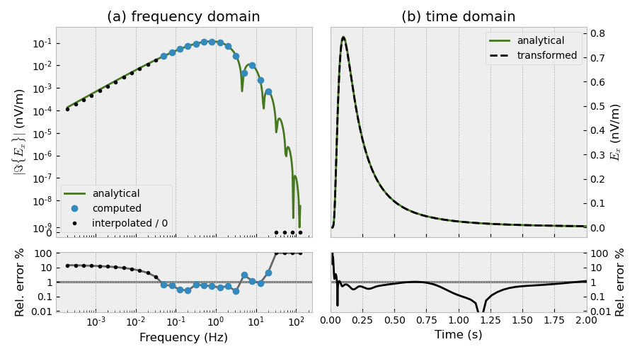
Plot it#
plt.figure(figsize=(9, 5), constrained_layout=True)

# Frequency-domain, imaginary, log-log
ax1 = plt.subplot2grid((4, 2), (0, 0), rowspan=3)
plt.title('(a) frequency domain')
plt.plot(freq_dense, 1e9*abs(epm_dense.imag), 'C3', label='analytical')
plt.plot(Fourier.freq_compute, 1e9*abs(data.imag), 'C0o', label='computed')
plt.plot(Fourier.freq_required[~Fourier.ifreq_compute],
         1e9*abs(data_int[~Fourier.ifreq_compute].imag), 'k.',
         label='interpolated / 0')
plt.ylabel(r'$|\Im\{E_x\}|$ (nV/m)')
plt.xscale('log')
plt.yscale('symlog', linthresh=5e-9)
plt.ylim([-1e-9, 5e-1])
ax1.set_xticklabels([])
plt.legend()
plt.grid(axis='y', c='0.9')

# Frequency-domain, imaginary, error
ax2 = plt.subplot2grid((4, 2), (3, 0))
plt.plot(Fourier.freq_required, err, '.4')
plt.plot(Fourier.freq_required[~Fourier.ifreq_compute],
         err[~Fourier.ifreq_compute], 'k.')
plt.plot(Fourier.freq_compute, err[Fourier.ifreq_compute], 'C0o')
plt.axhline(1, color='0.4', zorder=1)

plt.xscale('log')
plt.yscale('log')
plt.xlabel('Frequency (Hz)')
plt.ylabel('Rel. error %')
plt.ylim([8e-3, 120])
plt.yticks([0.01, 0.1, 1, 10, 100], ('0.01', '0.1', '1', '10', '100'))
plt.grid(axis='y', c='0.9')


# Time-domain
ax3 = plt.subplot2grid((4, 2), (0, 1), rowspan=3)
plt.title('(b) time domain')
plt.plot(time, epm_time*1e9, 'C3', lw=2, label='analytical')
plt.plot(time, data_time*1e9, 'k--', label='transformed')
plt.xlim([0, 2])
plt.ylabel('$E_x$ (nV/m)')
ax3.set_xticklabels([])
plt.legend()
ax3.yaxis.tick_right()
ax3.yaxis.set_label_position("right")
plt.grid(axis='y', c='0.9')

# Time-domain, error
ax4 = plt.subplot2grid((4, 2), (3, 1))
plt.plot(time, err_egd, 'k')
plt.axhline(1, color='0.4', zorder=1)

plt.yscale('log')
plt.xlabel('Time (s)')
plt.ylabel('Rel. error %')
plt.xlim([0, 2])
plt.ylim([8e-3, 120])
plt.yticks([0.01, 0.1, 1, 10, 100], ('0.01', '0.1', '1', '10', '100'))
ax4.yaxis.tick_right()
ax4.yaxis.set_label_position("right")
plt.grid(axis='y', c='0.9')
Total running time of the script: (0 minutes 49.751 seconds)
Estimated memory usage: 253 MB