Note
Go to the end to download the full example code.
GemPy-II: Perth Basin#
This example is mainly about building a deep marine resistivity model that can be used in other examples. There is not a lot of explanation. For more details regarding the integration of GemPy and emg3d see the GemPy-I: Simple Fault Model, and make sure to consult the many useful information over at GemPy.
The model is based on the Perth Basin Model from GemPy. We take the model, assign resistivities to the lithologies, create a random topography, move it 2 km down, fill it up with sea water, and add an air layer. The result is what is referred to in other examples as model GemPy-II, a synthetic, deep-marine resistivity model.
This model is used in, e.g., 03. Simulation.
Note
The original model (Perth_Basin) hosted on cgre-aachen/gempy_data is released under the LGPL-3.0 License.
import os
import emg3d
import pooch
from matplotlib.colors import LogNorm

# Adjust this path to a folder of your choice.
data_path = os.path.join('..', 'download', '')
Fetch the model#
Retrieve and load the pre-computed resistivity model.
fname = "GemPy-II.h5"
pooch.retrieve(
    'https://raw.github.com/emsig/data/2021-05-21/emg3d/models/'+fname,
    'ea8c23be80522d3ca8f36742c93758370df89188816f50cb4e1b2a6a3012d659',
    fname=fname,
    path=data_path,
)
fmodel = emg3d.load(data_path + fname)['model']
fgrid = fmodel.grid
Data loaded from «/home/dtr/Codes/emsig/emg3d-gallery/examples/download/GemPy-II.h5»
[emg3d v1.0.0rc3.dev5+g0cd9e09 (format 1.0) on 2021-05-21T18:40:16.721968].
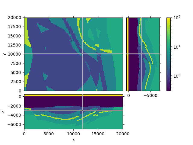
QC resistivity model#
fgrid.plot_3d_slicer(
    fmodel.property_x, zslice=-3000, xslice=12000,
    pcolor_opts={'norm': LogNorm(vmin=0.3, vmax=100)}
)
Reproduce the model#
Note
The following sections are about how to reproduce the model. For this you
have to install gempy. The code example and the GemPy-II.h5-file
used in the gallery were created on 2021-05-21 with gempy=2.2.9 and
pandas=1.2.4.
Get and initiate the Perth Basin#
import gempy as gempy
import numpy as np

# Initiate a model
geo_model = gempy.create_model('GemPy-II')
url_path = 'https://raw.githubusercontent.com/cgre-aachen/gempy_data/'
url_path += 'master/data/input_data/Perth_basin/'
path_i = "Paper_GU2F_sc_faults_topo_Points.csv"
path_o = "Paper_GU2F_sc_faults_topo_Foliations.csv"

pooch.retrieve(
    url_path + path_i,
    'f2964249dd941ceac35355beb78abd9c3189347fa6b845b6795240cc1a2f44d9',
    fname=path_i,
    path=data_path,
)
pooch.retrieve(
    url_path + path_o,
   'a6566d5caa8ce2fdcd4e4cb0ca643602436ca697342afacb31b7f4bd1d17c83d',
    fname=path_o,
    path=data_path,
)


# Define the grid
nx, ny, nz = 100, 100, 100
extent = [337000, 400000, 6640000, 6710000, -12000, 1000]

# Importing the data from CSV-files and setting extent and resolution
gempy.init_data(
    geo_model,
    extent=extent,
    resolution=[nx, ny, nz],
    path_i=data_path + "Paper_GU2F_sc_faults_topo_Points.csv",
    path_o=data_path + "Paper_GU2F_sc_faults_topo_Foliations.csv",
)
Initiate the stratigraphies and faults#
# We just follow the example here
del_surfaces = ['Cadda', 'Woodada_Kockatea', 'Cattamarra']
geo_model.delete_surfaces(del_surfaces)

# Map the different series
gempy.map_series_to_surfaces(
    geo_model,
    {
        "fault_Abrolhos_Transfer": ["Abrolhos_Transfer"],
        "fault_Coomallo": ["Coomallo"],
        "fault_Eneabba_South": ["Eneabba_South"],
        "fault_Hypo_fault_W": ["Hypo_fault_W"],
        "fault_Hypo_fault_E": ["Hypo_fault_E"],
        "fault_Urella_North": ["Urella_North"],
        "fault_Urella_South": ["Urella_South"],
        "fault_Darling": ["Darling"],
        "Sedimentary_Series": ['Cretaceous', 'Yarragadee', 'Eneabba',
                               'Lesueur', 'Permian']
    }
)

order_series = ["fault_Abrolhos_Transfer",
                "fault_Coomallo",
                "fault_Eneabba_South",
                "fault_Hypo_fault_W",
                "fault_Hypo_fault_E",
                "fault_Urella_North",
                "fault_Darling",
                "fault_Urella_South",
                "Sedimentary_Series",
                "Basement"]

_ = geo_model.reorder_series(order_series)

# Drop input data from the deleted series:
geo_model.surface_points.df.dropna(inplace=True)
geo_model.orientations.df.dropna(inplace=True)

# Set faults
geo_model.set_is_fault(["fault_Abrolhos_Transfer",
                        "fault_Coomallo",
                        "fault_Eneabba_South",
                        "fault_Hypo_fault_W",
                        "fault_Hypo_fault_E",
                        "fault_Urella_North",
                        "fault_Darling",
                        "fault_Urella_South"])
fr = geo_model.faults.faults_relations_df.values
fr[:, :-2] = False
_ = geo_model.set_fault_relation(fr)
Compute the model with GemPy#
# Set the interpolator.
gempy.set_interpolator(
    geo_model,
    compile_theano=True,
    theano_optimizer='fast_run',
    gradient=False,
    dtype='float32',
    verbose=[]
)

# Compute it.
sol = gempy.compute_model(geo_model, compute_mesh=True)

# Get the solution at the internal grid points.
sol = gempy.compute_model(geo_model)
Assign resistivities to the id’s#
We define here a discretize mesh identical to the mesh used by GemPy, and subsequently assign resistivities to the different lithologies.
Please note that these resistivities are made up, and do not necessarily relate to the actual lithologies.
# We create a mesh 20 km x 20 km x 5 km, starting at the origin.
# As long as we have the same number of cells we can trick the grid
# original into any grid we want.
hx = np.ones(nx)*20000/nx
hy = np.ones(ny)*20000/ny
hz = np.ones(nz)*5000/nz
grid = emg3d.TensorMesh([hx, hy, hz], origin=(0, 0, -5000))

# Make up some resistivities that might be interesting to model.
ids = np.round(sol.lith_block)
res = np.ones(grid.n_cells)
res[ids == 9] = 2.0    # Cretaceous
res[ids == 10] = 1.0   # Yarragadee
res[ids == 11] = 4.0   # Eneabba
res[ids == 12] = 50.0  # Lesueur
res[ids == 13] = 7.0   # Permian
res[ids == 14] = 10.0  # Basement
Topography#
Calls to geo_model.set_topography(source='random') create a random
topography every time. In order to have it reproducible we saved it once and
load it now.
Originally it was created and stored like this:
out = geo_model.set_topography(source='random')
np.save(data_path + topo_name, topo)
# Load the stored topography.
topo_name = 'GemPy-II-topo.npy'
topo_path = 'https://raw.github.com/emsig/data/2021-05-21/'
topo_path += 'emg3d/external/GemPy/'+topo_name

pooch.retrieve(
    topo_path,
    '10bb3d672ba26f6d8cb85eb33086daebb1c19bcbf9547c0b17d93f1c0dcf4e20',
    fname=topo_name,
    path=data_path,
)

out = geo_model.set_topography(
        source='saved', filepath=data_path+topo_name, allow_pickle=True)
topo = out.topography.values_2d

# Apply the topography to our resistivity cube.
res = res.reshape(grid.shape_cells, order='C')

# Get the scaling factor betw. original extent and our made-up extent.
fact = 5000/np.diff(extent[4:])

# Loop over all x-y-values and convert cells above topography to water.
for ix in range(nx):
    for iy in range(ny):
        res[ix, iy, grid.cell_centers_z > topo[ix, iy, 2]*fact] = 0.3
Extend the model by sea water and air#
# Create an emg3d-model.
model = emg3d.Model(grid, property_x=res.ravel('F'))

# Add 2 km water and 500 m air.
fhz = np.r_[np.ones(nz)*5000/nz, 2000, 500]
z0 = -7000

# Make the full mesh
fgrid = emg3d.TensorMesh([hx, hy, fhz], origin=(0, 0, z0))

# Extend the model.
fmodel = emg3d.Model(fgrid, np.ones(fgrid.shape_cells))
fmodel.property_x[:, :, :-2] = model.property_x
fmodel.property_x[:, :, -2] = 0.3
fmodel.property_x[:, :, -1] = 1e8

# emg3d.save(data_path + 'GemPy-II.h5', model=fmodel)

fgrid
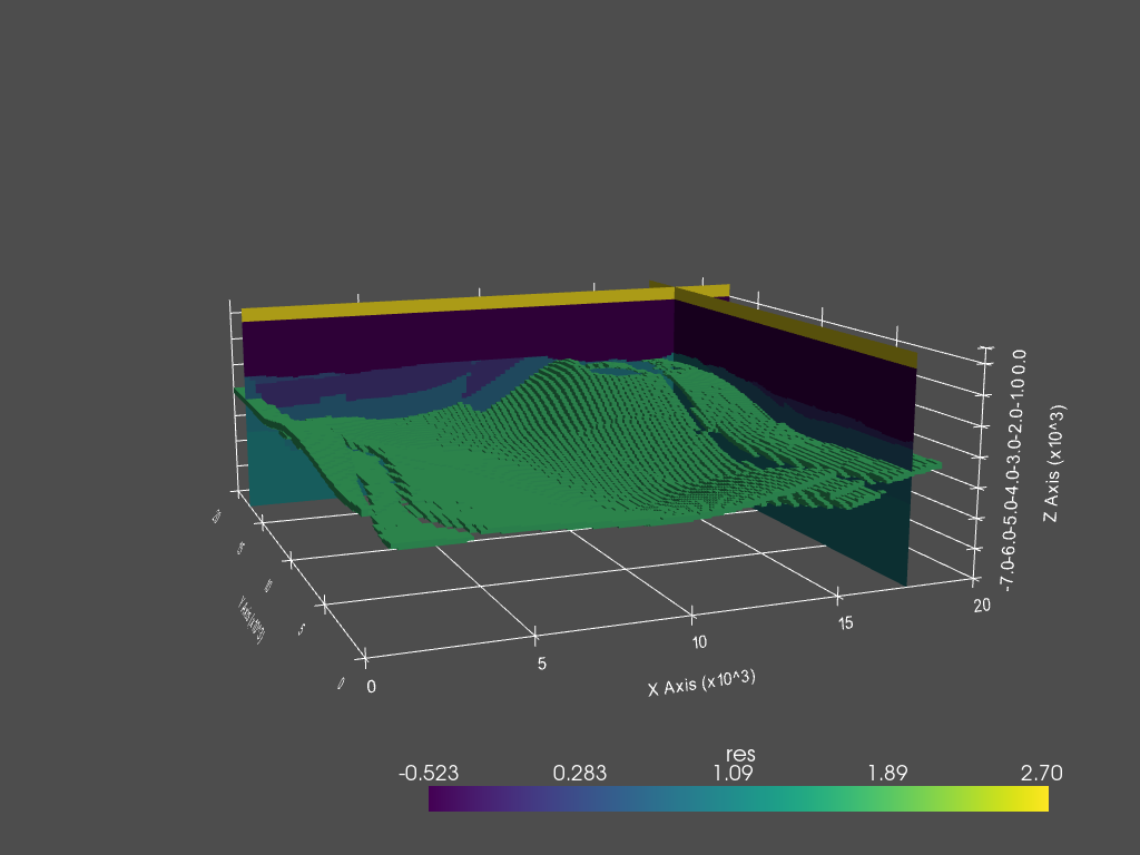
PyVista plot#
Note
The final cell is about how to plot the model in 3D using PyVista,
for which you have to install pyvista.
The code example was created on 2021-05-21 with pyvista=0.30.1.
import pyvista
import numpy as np

dataset = fgrid.toVTK({'res': np.log10(fmodel.property_x.ravel('F'))})

# Create the rendering scene and add a grid axes
p = pyvista.Plotter(notebook=True)
p.show_grid(location='outer')

# Add spatially referenced data to the scene
dparams = {'rng': np.log10([0.3, 500]), 'show_edges': False}
xyz = (17500, 17500, -1500)
p.add_mesh(dataset.slice('x', xyz), name='x-slice', **dparams)
p.add_mesh(dataset.slice('y', xyz), name='y-slice', **dparams)

# Add a layer as 3D
p.add_mesh(dataset.threshold(
    [np.log10(49.9), np.log10(50.1)]), name='vol', **dparams)

# Show the scene!
p.camera_position = [
      (-10000, -41000, 8500), (10000, 10000, -3250), (0, 0, 1)
]
p.show()
Total running time of the script: (0 minutes 1.227 seconds)
Estimated memory usage: 229 MB