06. Parameter tests

The modeller emg3d has quite a few parameters which can influence the speed of a computation. It can be difficult to estimate which is the best setting. In the case that speed is of utmost importance, and a lot of similar models are going to be computed (e.g. for inversions), it might be worth to do some input parameter testing.

IMPORTANT: None of the conclusions you can draw from these figures are applicable to other models. What is faster depends on your input. Influence has particularly the degree of anisotropy and of grid stretching. These are simply examples that you can adjust for your problem at hand.

import emg3d
import numpy as np
import matplotlib.pyplot as plt
from matplotlib.colors import LogNorm
plt.style.use('bmh')

def plotit(infos, labels):
    """Simple plotting routine for the tests."""

    plt.figure()

    # Loop over infos.
    for i, info in enumerate(infos):
        plt.plot(info['runtime_at_cycle'],
                 info['error_at_cycle']/info1['ref_error'],
                 '.-', label=labels[i])

    plt.legend()
    plt.xlabel('Time (s)')
    plt.ylabel('Rel. Error $(-)$')
    plt.yscale('log')

    plt.show()

# Survey
zwater = 1000                  # Water depth.
src = [0, 0, 50-zwater, 0, 0]  # Source at origin, 50 m above seafloor.
freq = 1.0                     # Frequency (Hz).

# Mesh
grid = emg3d.construct_mesh(
    frequency=freq,
    min_width_limits=100,
    properties=[0.3, 1., 1., 0.3],
    center=(src[0], src[1], -1000),
    domain=([-1000, 5000], [-500, 500], [-2500, 0]),
    center_on_edge=False,
)
print(grid)

# Source-field
sfield = emg3d.get_source_field(grid, source=src, frequency=freq)

# Create a simple marine model for the tests.

# Layered_background
res_x = 1e8*np.ones(grid.shape_cells)              # Air
res_x[:, :, grid.cell_centers_z <= 0] = 0.3     # Water
res_x[:, :, grid.cell_centers_z <= -1000] = 1.  # Background

# Target
xt = np.nonzero((grid.cell_centers_x >= -500) &
                (grid.cell_centers_x <= 5000))[0]
yt = np.nonzero((grid.cell_centers_y >= -1000) &
                (grid.cell_centers_y <= 1000))[0]
zt = np.nonzero((grid.cell_centers_z >= -2100) &
                (grid.cell_centers_z <= -1800))[0]
res_x[xt[0]:xt[-1]+1, yt[0]:yt[-1]+1, zt[0]:zt[-1]+1] = 100

# Create a model instance
model_iso = emg3d.Model(grid, property_x=res_x, mapping='Resistivity')

# Plot it for QC
grid.plot_3d_slicer(model_iso.property_x.ravel('F'),
                    pcolor_opts={'norm': LogNorm()})

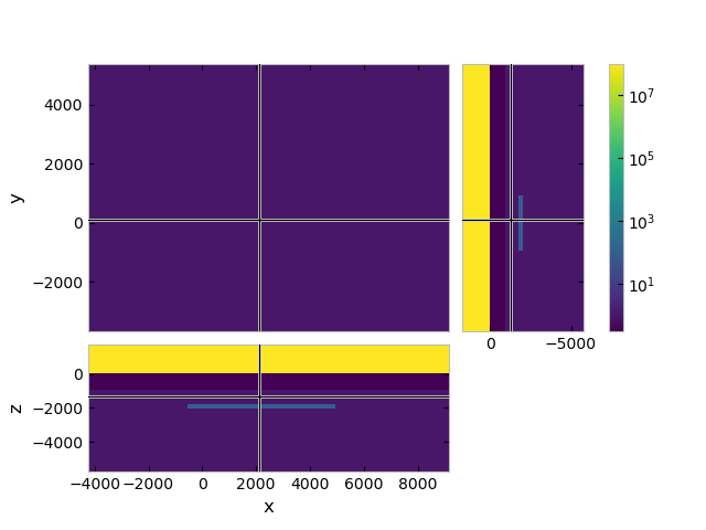
TensorMesh: 76,800 cells

                    MESH EXTENT             CELL WIDTH      FACTOR
dir    nC        min           max         min       max      max
---   ---  ---------------------------  ------------------  ------
 x     80     -4,233.88      9,146.56    100.00    912.68    1.25
 y     24     -3,667.19      5,375.78    100.00  1,708.59    1.50
 z     40     -5,764.95      1,752.46    100.00    857.19    1.31

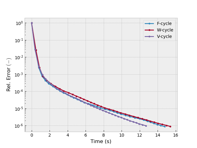
Test 1: F, W, and V MG cycles

inp = {'model': model_iso, 'sfield': sfield, 'return_info': True,
       'sslsolver': False, 'semicoarsening': False, 'linerelaxation': False}

_, info1 = emg3d.solve(cycle='F', **inp)
_, info2 = emg3d.solve(cycle='W', **inp)
_, info3 = emg3d.solve(cycle='V', **inp)

plotit([info1, info2, info3], ['F-cycle', 'W-cycle', 'V-cycle'])

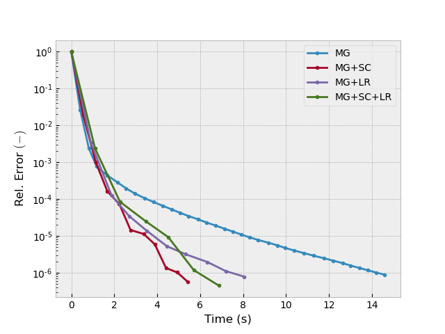
Test 2: semicoarsening, line-relaxation

inp = {'model': model_iso, 'sfield': sfield, 'return_info': True,
       'sslsolver': False}

_, info1 = emg3d.solve(semicoarsening=False, linerelaxation=False, **inp)
_, info2 = emg3d.solve(semicoarsening=True, linerelaxation=False, **inp)
_, info3 = emg3d.solve(semicoarsening=False, linerelaxation=True, **inp)
_, info4 = emg3d.solve(semicoarsening=True, linerelaxation=True, **inp)

plotit([info1, info2, info3, info4], ['MG', 'MG+SC', 'MG+LR', 'MG+SC+LR'])

Test 3: MG and BiCGstab

inp = {'model': model_iso, 'sfield': sfield, 'return_info': True, 'maxit': 500,
       'semicoarsening': True, 'linerelaxation': False}

_, info1 = emg3d.solve(cycle='F', sslsolver=False, **inp)
_, info2 = emg3d.solve(cycle='F', sslsolver=True, **inp)
_, info3 = emg3d.solve(cycle=None, sslsolver=True, **inp)

plotit([info1, info2, info3], ['MG', 'MG+BiCGStab', 'BiCGStab'])

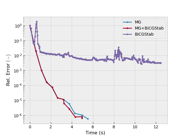
* WARNING :: Error in bicgstab (-10)

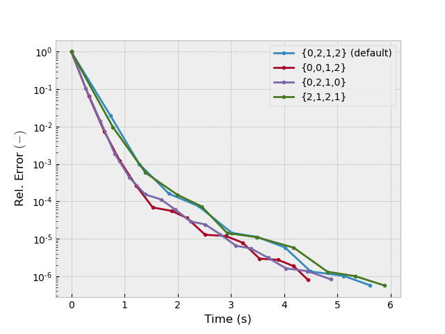
Test 4: nu_init, nu_pre, nu_coarse, nu_post

inp = {'model': model_iso, 'sfield': sfield, 'return_info': True,
       'sslsolver': False, 'semicoarsening': True, 'linerelaxation': False}

_, info1 = emg3d.solve(**inp)
_, info2 = emg3d.solve(nu_pre=0, **inp)
_, info3 = emg3d.solve(nu_post=0, **inp)
_, info4 = emg3d.solve(nu_init=2, **inp)

plotit([info1, info2, info3, info4],
       ['{0,2,1,2} (default)', '{0,0,1,2}', '{0,2,1,0}', '{2,1,2,1}'])

emg3d.Report()

Wed Aug 31 21:34:41 2022 CEST
OS	Linux	CPU(s)	4	Machine	x86_64
Architecture	64bit	RAM	15.5 GiB	Environment	Python
File system	ext4
Python 3.9.12 | packaged by conda-forge | (main, Mar 24 2022, 23:22:55) [GCC 10.3.0]
numpy	1.22.4	scipy	1.9.0	numba	0.55.2
emg3d	1.8.0	empymod	2.2.0	xarray	2022.6.0
discretize	0.8.2	h5py	3.7.0	matplotlib	3.4.3
tqdm	4.64.0	IPython	8.4.0
Intel(R) oneAPI Math Kernel Library Version 2022.0-Product Build 20211112 for Intel(R) 64 architecture applications

Estimated memory usage: 59 MB