Note
Go to the end to download the full example code.
7. Magnetic source using an electric loop#
Computing the \(E\) and \(H\) fields generated by a magnetic source
We know that we can get the magnetic fields from the electric fields using Faraday’s law, see 6. Magnetic field due to an el. source.
However, what about computing the fields generated by a magnetic source? There are two ways we can achieve that:
creating an electric loop source, which is what we do in this example, or
using the duality principle, see 8. Magnetic source using duality.
We create a “magnetic dipole” through an electric loop perpendicular to the
defined dipole in a homogeneous VTI fullspace, and compare it to the
semi-analytical solution of empymod. (The code empymod is an
open-source code which can model CSEM responses for a layered medium including
VTI electrical anisotropy, see emsig.xyz.)
import emg3d
import empymod
import numpy as np
import matplotlib.pyplot as plt
Full-space model for a loop dipole#
In order to shorten the build-time of the gallery we use a coarse model.
Set coarse_model = False to obtain a result of higher accuracy.
coarse_model = True
Survey and model parameters#
emg3d.TxMagneticDipole creates an electric square loop perpendicular to
the defined dipole, where the area of the square loop corresponds to the
length of the dipole.
# Receiver coordinates
if coarse_model:
    x = (np.arange(256))*20-2550
else:
    x = (np.arange(1025))*5-2560
rx = np.repeat([x, ], np.size(x), axis=0)
ry = rx.transpose()
frx, fry = rx.ravel(), ry.ravel()
rz = -400.0
azimuth = 25
elevation = 10

# Source coordinates, frequency, and strength
source = emg3d.TxMagneticDipole(
    coordinates=[-0.5, 0.5, -0.3, 0.3, -300.5, -299.5],  # [x1,x2,y1,y2,z1,z2]
    strength=np.pi,  # A
)
frequency = 0.77  # Hz

# Model parameters
h_res = 1.              # Horizontal resistivity
aniso = np.sqrt(2.)     # Anisotropy
v_res = h_res*aniso**2  # Vertical resistivity
empymod#
Note: The coordinate system of empymod is positive z down, for emg3d it is positive z up. We have to switch therefore src_z, rec_z, and elevation.
# Collect common input for empymod.
inp = {
    'src': np.r_[source.coordinates[:4], -source.coordinates[4:]],
    'depth': [],
    'res': h_res,
    'aniso': aniso,
    'strength': source.strength,
    'freqtime': frequency,
    'htarg': {'pts_per_dec': -1},
}

# Compute e-field
epm_e = -empymod.loop(
    rec=[frx, fry, -rz, azimuth, -elevation], mrec=False, verb=3, **inp
).reshape(np.shape(rx))

# Compute h-field
epm_h = -empymod.loop(
    rec=[frx, fry, -rz, azimuth, -elevation], **inp
).reshape(np.shape(rx))
:: empymod START  ::  v2.6.0

   depth       [m] :
   res     [Ohm.m] :  1
   aniso       [-] :  1.41421
   epermH      [-] :  1
   epermV      [-] :  1
   mpermH      [-] :  1
   mpermV      [-] :  1

>  MODEL IS A FULLSPACE
   direct field    :  Comp. in wavenumber domain
   frequency  [Hz] :  0.77
   Hankel          :  DLF (Fast Hankel Transform)
     > Filter      :  key_201_2009
     > DLF type    :  Lagged Convolution
   Loop over       :  Frequencies
   Source type     :  Magnetic flux
   Receiver type   :  Electric field
   Source(s)       :  1 dipole(s)
     > intpts      :  1 (as dipole)
     > length  [m] :  1.53623
     > strength[A] :  3.14159
     > x_c     [m] :  0
     > y_c     [m] :  0
     > z_c     [m] :  300
     > azimuth [°] :  30.9638
     > dip     [°] :  -40.6129
   Receiver(s)     :  65536 dipole(s)
     > x       [m] :  -2550 - 2550 : 65536  [min-max; #]
     > y       [m] :  -2550 - 2550 : 65536  [min-max; #]
     > z       [m] :  400
     > azimuth [°] :  25
     > dip     [°] :  -10
   Required ab's   :  14 15 16 24 25 26 34 35 36

:: empymod END; runtime = 0:00:00.067071 :: 8 kernel call(s)


:: empymod END; runtime = 0:00:00.063760 :: 9 kernel call(s)
emg3d#
if coarse_model:
    min_width_limits = 40
    stretching = [1.045, 1.045]
else:
    min_width_limits = 20
    stretching = [1.03, 1.045]

# Create stretched grid
grid = emg3d.construct_mesh(
    frequency=frequency,
    properties=h_res,
    center=source.center,
    domain=([-2500, 2500], [-2500, 2500], [-2900, 2100]),
    min_width_limits=min_width_limits,
    stretching=stretching,
    lambda_from_center=True,
    lambda_factor=0.8,
    center_on_edge=False,
)
grid
:: emg3d START :: 21:54:38 :: v1.8.7

   MG-cycle       : 'F'                 sslsolver : False
   semicoarsening : False [0]           tol       : 1e-06
   linerelaxation : False [0]           maxit     : 50
   nu_{i,1,c,2}   : 0, 2, 1, 2          verb      : 4
   Original grid  :  80 x  80 x  80     => 512,000 cells
   Coarsest grid  :   5 x   5 x   5     => 125 cells
   Coarsest level :   4 ;   4 ;   4

   [hh:mm:ss]  rel. error                  [abs. error, last/prev]   l s

       h_
      2h_ \                  /
      4h_  \          /\    /
      8h_   \    /\  /  \  /
     16h_    \/\/  \/    \/

   [21:54:39]   4.451e-03  after   1 F-cycles   [4.617e-09, 0.004]   0 0
   [21:54:40]   1.643e-04  after   2 F-cycles   [1.704e-10, 0.037]   0 0
   [21:54:41]   8.138e-06  after   3 F-cycles   [8.443e-12, 0.050]   0 0
   [21:54:42]   4.803e-07  after   4 F-cycles   [4.983e-13, 0.059]   0 0

   > CONVERGED
   > MG cycles        : 4
   > Final rel. error : 4.803e-07

:: emg3d END   :: 21:54:42 :: runtime = 0:00:04
Plot function#
def plot(epm, e3d, title, vmin, vmax):

    # Start figure.
    a_kwargs = {'cmap': "viridis", 'vmin': vmin, 'vmax': vmax,
                'shading': 'nearest'}

    e_kwargs = {'cmap': plt.get_cmap("RdBu_r", 8),
                'vmin': -2, 'vmax': 2, 'shading': 'nearest'}

    fig, axs = plt.subplots(2, 3, figsize=(10, 5.5), sharex=True, sharey=True,
                            subplot_kw={'box_aspect': 1})

    ((ax1, ax2, ax3), (ax4, ax5, ax6)) = axs
    x3 = x/1000  # km

    # Plot Re(data)
    ax1.set_title(r"(a) |Re(empymod)|")
    cf0 = ax1.pcolormesh(x3, x3, np.log10(epm.real.amp()), **a_kwargs)

    ax2.set_title(r"(b) |Re(emg3d)|")
    ax2.pcolormesh(x3, x3, np.log10(e3d.real.amp()), **a_kwargs)

    ax3.set_title(r"(c) Error real part")
    rel_error = 100*np.abs((epm.real - e3d.real) / epm.real)
    cf2 = ax3.pcolormesh(x3, x3, np.log10(rel_error), **e_kwargs)

    # Plot Im(data)
    ax4.set_title(r"(d) |Im(empymod)|")
    ax4.pcolormesh(x3, x3, np.log10(epm.imag.amp()), **a_kwargs)

    ax5.set_title(r"(e) |Im(emg3d)|")
    ax5.pcolormesh(x3, x3, np.log10(e3d.imag.amp()), **a_kwargs)

    ax6.set_title(r"(f) Error imaginary part")
    rel_error = 100*np.abs((epm.imag - e3d.imag) / epm.imag)
    ax6.pcolormesh(x3, x3, np.log10(rel_error), **e_kwargs)

    # Colorbars
    unit = "(V/m)" if "E" in title else "(A/m)"
    fig.colorbar(cf0, ax=axs[0, :], label=r"$\log_{10}$ Amplitude "+unit)
    cbar = fig.colorbar(cf2, ax=axs[1, :], label=r"Relative Error")
    cbar.set_ticks([-2, -1, 0, 1, 2])
    cbar.ax.set_yticklabels([r"$0.01\,\%$", r"$0.1\,\%$", r"$1\,\%$",
                             r"$10\,\%$", r"$100\,\%$"])

    ax1.set_xlim(min(x3), max(x3))
    ax1.set_ylim(min(x3), max(x3))

    # Axis label
    fig.text(0.4, 0.05, "Inline Offset (km)", fontsize=14)
    fig.text(0.05, 0.3, "Crossline Offset (km)", rotation=90, fontsize=14)
    fig.suptitle(title, y=1, fontsize=20)

    print(f"- Source: {source}")
    print(f"- Frequency: {frequency} Hz")
    rtype = "Electric" if "E" in title else "Magnetic"
    print(f"- {rtype} receivers: z={rz} m; θ={azimuth}°, φ={elevation}°")
Compare the electric field generated from the magnetic source#
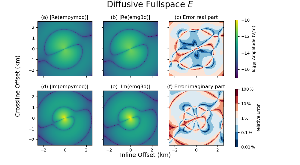
- Source: TxMagneticDipole: 3.1 A;
    e1={-0.5; -0.3; -300.5} m; e2={0.5; 0.3; -299.5} m
- Frequency: 0.77 Hz
- Electric receivers: z=-400.0 m; θ=25°, φ=10°
Compare the magnetic field generated from the magnetic source#
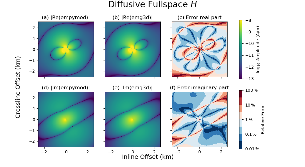
- Source: TxMagneticDipole: 3.1 A;
    e1={-0.5; -0.3; -300.5} m; e2={0.5; 0.3; -299.5} m
- Frequency: 0.77 Hz
- Magnetic receivers: z=-400.0 m; θ=25°, φ=10°
Total running time of the script: (0 minutes 7.400 seconds)
Estimated memory usage: 311 MB