Note
Go to the end to download the full example code.
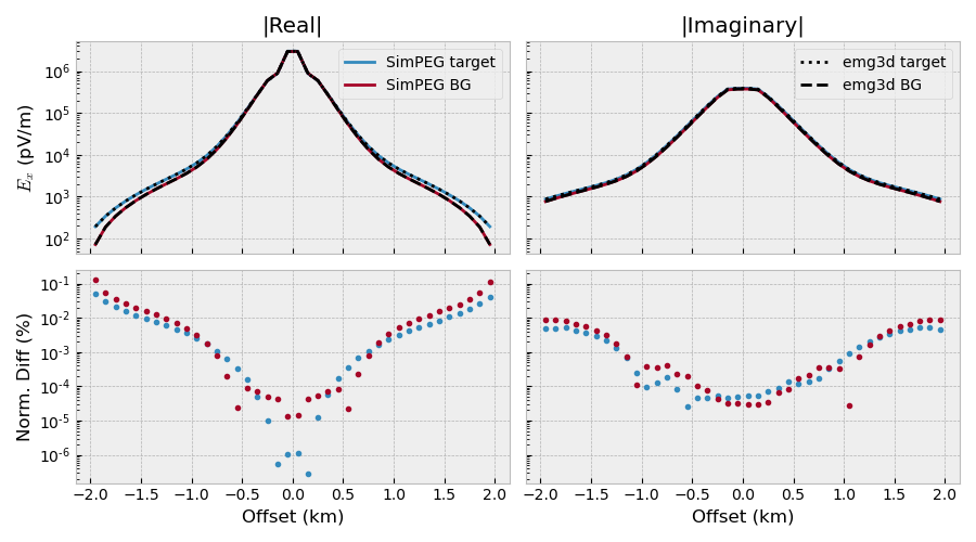
3. SimPEG: 3D with tri-axial anisotropy#
SimPEG is an open source python package for simulation
and gradient based parameter estimation in geophysical applications. Here we
compare emg3d with SimPEG using the forward solver Pardiso.
import os
import pooch
import emg3d
import numpy as np
import matplotlib.pyplot as plt
plt.style.use('bmh')


# Adjust this path to a folder of your choice.
data_path = os.path.join('..', 'download', '')
Model parameters#
# Depths (0 is sea-surface);
# hence a deep sea case where we can ignore the air.
water_depth = 3000
target_x = np.r_[-500, 500]
target_y = target_x
target_z = -water_depth + np.r_[-400, -100]

# Resistivities
res_sea = 0.33
res_back = [1., 2., 3.]  # Background in x-, y-, and z-directions
res_target = 100.

# Acquisition frequency
frequency = 1.0
Grid#
Survey parameters#
# We take the receiver locations at the actual CCx-locations
rec_x = grid.cell_centers_x[12:-12]
rec = (rec_x, 0, -water_depth, 0, 0)
print(f"Receiver locations:\n{rec_x}\n")

source = emg3d.TxElectricDipole([-100, 100, 0, 0, -2900, -2900])
sfield = emg3d.get_source_field(grid, source, frequency)  # Source field
Receiver locations:
[-1950. -1850. -1750. -1650. -1550. -1450. -1350. -1250. -1150. -1050.
  -950.  -850.  -750.  -650.  -550.  -450.  -350.  -250.  -150.   -50.
    50.   150.   250.   350.   450.   550.   650.   750.   850.   950.
  1050.  1150.  1250.  1350.  1450.  1550.  1650.  1750.  1850.  1950.]
Create model#
# Layered_background
res_x = res_sea*np.ones(grid.n_cells)
res_y = res_x.copy()
res_z = res_x.copy()
# Tri-axial background.
res_x[grid.cell_centers[:, 2] <= -water_depth] = res_back[0]
res_y[grid.cell_centers[:, 2] <= -water_depth] = res_back[1]
res_z[grid.cell_centers[:, 2] <= -water_depth] = res_back[2]
res_x_bg = res_x.copy()
res_y_bg = res_y.copy()
res_z_bg = res_z.copy()
# Include the target
target_inds = (
(grid.cell_centers[:, 0] >= target_x[0]) &
(grid.cell_centers[:, 0] <= target_x[1]) &
(grid.cell_centers[:, 1] >= target_y[0]) &
(grid.cell_centers[:, 1] <= target_y[1]) &
(grid.cell_centers[:, 2] >= target_z[0]) &
(grid.cell_centers[:, 2] <= target_z[1])
)
res_x[target_inds] = res_target
res_y[target_inds] = res_target
res_z[target_inds] = res_target
# Create emg3d-models for given frequency
model = emg3d.Model(
grid, property_x=res_x, property_y=res_y,
property_z=res_z, mapping='Resistivity')
model_bg = emg3d.Model(
grid, property_x=res_x_bg, property_y=res_y_bg,
property_z=res_z_bg, mapping='Resistivity')
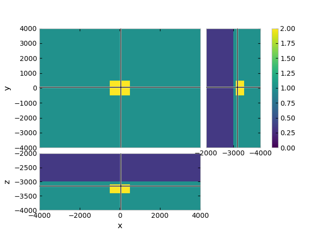
# Plot a slice
grid.plot_3d_slicer(
model.property_x, zslice=-3200, clim=[0, 2],
xlim=(-4000, 4000), ylim=(-4000, 4000), zlim=(-4000, -2000)
)
Compute emg3d#
e3d_ftg = emg3d.solve(model, sfield, verb=1)
e3d_tg = e3d_ftg.get_receiver(rec)

e3d_fbg = emg3d.solve(model_bg, sfield, verb=1)
e3d_bg = e3d_fbg.get_receiver(rec)
:: emg3d :: 7.2e-07; 1(4); 0:00:03; CONVERGED
:: emg3d :: 6.6e-07; 1(4); 0:00:03; CONVERGED
Fetch and load SimPEG result#
# Fetch pre-computed data.
fname = 'simpeg.h5'
pooch.retrieve(
    'https://raw.github.com/emsig/data/2021-05-21/emg3d/external/'+fname,
    'e0502ccfb6dfec599f4c53d9b8f8a0c79b7d872c7224a9b403cb57f39e729409',
    fname=fname,
    path=data_path,
)

# Load pre-computed data.
spg = emg3d.load(data_path + fname)
spg_tg, spg_bg = spg['spg_tg'], spg['spg_bg']
Data loaded from «/home/dtr/Codes/emsig/emg3d-gallery/examples/download/simpeg.h5»
[emg3d v0.17.1.dev22+ge23c468 (format 1.0) on 2021-04-15T16:28:20.499498].
Plot result#
def nrmsd(a, b):
    """Return Normalized Root-Mean-Square Difference."""
    return 200 * abs(a - b) / (abs(a) + abs(b))


fig, axs = plt.subplots(
        2, 2, figsize=(9, 5), sharex=True, sharey='row',
        constrained_layout=True)
((ax1, ax3), (ax2, ax4)) = axs

# Real part
ax1.set_title(r'|Real|')
ax1.plot(rec_x/1e3, 1e12*np.abs(spg_tg.real), 'C0-', label='SimPEG target')
ax1.plot(rec_x/1e3, 1e12*np.abs(spg_bg.real), 'C1-', label='SimPEG BG')
ax1.plot(rec_x/1e3, 1e12*np.abs(e3d_tg.real), 'k:')
ax1.plot(rec_x/1e3, 1e12*np.abs(e3d_bg.real), 'k--')
ax1.set_ylabel('$E_x$ (pV/m)')
ax1.set_yscale('log')
ax1.legend()

# Normalized difference real
ax2.plot(rec_x/1e3, nrmsd(spg_tg.real, e3d_tg.real), 'C0.')
ax2.plot(rec_x/1e3, nrmsd(spg_bg.real, e3d_bg.real), 'C1.')
ax2.set_ylabel('Norm. Diff (%)')
ax2.set_xlabel('Offset (km)')

# Imaginary part
ax3.set_title(r'|Imaginary|')
ax3.plot(rec_x/1e3, 1e12*np.abs(spg_tg.imag), 'C0-')
ax3.plot(rec_x/1e3, 1e12*np.abs(spg_bg.imag), 'C1-')
ax3.plot(rec_x/1e3, 1e12*np.abs(e3d_tg.imag), 'k:', label='emg3d target')
ax3.plot(rec_x/1e3, 1e12*np.abs(e3d_bg.imag), 'k--', label='emg3d BG')
ax3.legend()

# Normalized difference imag
ax4.plot(rec_x/1e3, nrmsd(spg_tg.imag, e3d_tg.imag), 'C0.')
ax4.plot(rec_x/1e3, nrmsd(spg_bg.imag, e3d_bg.imag), 'C1.')
ax4.set_xlabel('Offset (km)')
ax4.set_yscale('log')
Reproduce SimPEG result#
In order to reduce (a) the number of dependencies to generate the gallery and, more importantly, (b) the runtime and memory requirements of the gallery the SimPEG result is pre-computed.
Note
The following cell needs to be carried out to compute the SimPEG results
from scratch. For this you have to install simpeg and
pymatsolver. The code example and the simpeg.h5-file used above
were created on 2021-04-14 with simpeg=0.14.3, pymatsolver=0.1.1,
and discretize=0.6.3.
# Note, in order to use the ``Pardiso``-solver ``pymatsolver`` has to be
# installed via ``conda``, not via ``pip``!
import SimPEG
import discretize
import pymatsolver
import SimPEG.electromagnetics.frequency_domain as FDEM

# Set up the receivers
rx_locs = discretize.utils.ndgrid([rec_x, np.r_[0], np.r_[-water_depth]])
rx_list = [
    FDEM.receivers.PointElectricField(
        orientation='x', component="real", locations=rx_locs),
    FDEM.receivers.PointElectricField(
        orientation='x', component="imag", locations=rx_locs)
]

# We use the emg3d-source-vector, to ensure we use the same in both cases
svector = np.real(sfield.field/-sfield.smu0)
src_sp = FDEM.sources.RawVec_e(rx_list, s_e=svector, frequency=frequency)
src_list = [src_sp]
survey = FDEM.Survey(src_list)

# Define the Simulation
mesh = discretize.TensorMesh(grid.h, grid.origin)
sim = FDEM.simulation.Simulation3DElectricField(
        mesh,
        survey=survey,
        sigmaMap=SimPEG.maps.IdentityMap(mesh),
        solver=pymatsolver.Pardiso,
)

spg_tg_dobs = sim.dpred(np.vstack([1./res_x, 1./res_y, 1./res_z]).T)
spg_ftg = SimPEG.survey.Data(survey, dobs=spg_tg_dobs)

spg_bg_dobs = sim.dpred(
        np.vstack([1./res_x_bg, 1./res_y_bg, 1./res_z_bg]).T)
spg_fbg = SimPEG.survey.Data(survey, dobs=spg_bg_dobs)

spg_tg = spg_ftg[src_sp, rx_list[0]] + 1j*spg_ftg[src_sp, rx_list[1]]
spg_bg = spg_fbg[src_sp, rx_list[0]] + 1j*spg_fbg[src_sp, rx_list[1]]

# emg3d.save('simpeg.h5', spg_tg=spg_tg, spg_bg=spg_bg)
Total running time of the script: (0 minutes 9.160 seconds)
Estimated memory usage: 248 MB