Note
Go to the end to download the full example code.
08. Ensure computation domain is big enough#
Ensure the boundary in \(\pm x\), \(\pm y\), and \(+ z\) is big enough for \(\rho_\text{air}\).
The air is very resistive, and EM waves propagate at the speed of light as a wave, not diffusive any longer. The whole concept of skin depth does therefore not apply to the air layer. The only attenuation is caused by geometrical spreading. In order to not have any effects from the boundary one has to choose the air layer appropriately.
The important bit is that the resistivity of air has to be taken into account also for the horizontal directions, not only for positive \(z\) (upwards into the sky). This is an example to test boundaries on a simple marine model (air, water, subsurface) and compare them to the 1D result.
import emg3d
import empymod
import numpy as np
import matplotlib.pyplot as plt
from matplotlib.colors import LogNorm
plt.style.use('ggplot')
Model, Survey, and Analytical Solution#
water_depth = 500                        # 500 m water depth
offsets = np.linspace(2000, 7000, 501)   # Offsets
src_coo = [0, 0, -water_depth+50, 0, 0]  # Src at origin, 50 m above seafloor
rec_coo = [offsets, offsets*0, -water_depth, 0, 0]  # Receivers on the seafloor
depth = [-water_depth, 0]                # Simple model
resistivity = [1, 0.3, 1e8]              # Simple model
frequency = 0.1                          # Frequency

source = emg3d.TxElectricDipole(src_coo)

# Compute analytical solution
epm = empymod.bipole(src_coo, rec_coo, depth, resistivity, frequency)
:: empymod END; runtime = 0:00:06.792336 :: 1 kernel call(s)
3D Modelling#
# Parameter we keep the same for both grids
grid_inp = {
    'frequency': frequency,
    'center': [src_coo[0], src_coo[1], -water_depth-100],
    'domain': ([src_coo[0]-500, offsets[-1]+500],
               [src_coo[1], src_coo[1]],
               [-600, 100]),
    'seasurface': 0,
    'min_width_limits': 100,
    'stretching': [1, 1.25],
    'lambda_from_center': True,
    'center_on_edge': True,
    'verb': 1,
}
1st grid, only considering air resistivity for +z#
Here we are in the water, so the signal is attenuated before it enters the air. So we don’t use the resistivity of air to compute the required boundary, but 100 Ohm.m instead. (100 is the result of a quick parameter test with \(\rho=1e4, 1e3, 1e2, 1e1\), and the result was that after 100 there is not much improvement any longer.)
Also note that the function emg3d.meshes.construct_mesh() internally
uses six times the skin depth for the boundary. For \(\rho\) = 100 Ohm.m
and \(f\) = 0.1 Hz, the skin depth \(\delta\) is roughly 16 km, which
therefore results in a boundary of roughly 96 km.
See the documentation of emg3d.meshes.get_hx_h0() for more information
on how the grid is created.
         == GRIDDING IN X ==
Skin depth     [m] : 872 / 1592 / 1592  [corr. to `properties`]
Survey dom. DS [m] : -500 - 7500
Comp. dom. DC  [m] : -10250 - 13750
Final extent   [m] : -10405 - 14205
Cell widths    [m] : 100 / 100 / 904  [min(DS) / max(DS) / max(DC)]
Number of cells    : 128 (80 / 48 / 0)  [Total (DS/DC/remain)]
Max stretching     : 1.000 (1.000) / 1.088  [DS (seasurface) / DC]

         == GRIDDING IN Y ==
Skin depth     [m] : 872 / 1592 / 1592  [corr. to `properties`]
Survey dom. DS [m] : 0 - 0
Comp. dom. DC  [m] : -10000 - 10000
Final extent   [m] : -10226 - 10226
Cell widths    [m] : 100 / 100 / 1907  [min(DS) / max(DS) / max(DC)]
Number of cells    : 32 (2 / 30 / 0)  [Total (DS/DC/remain)]
Max stretching     : 1.000 (1.000) / 1.217  [DS (seasurface) / DC]

         == GRIDDING IN Z ==
Skin depth     [m] : 872 / 1592 / 15915  [corr. to `properties`]
Survey dom. DS [m] : -600 - 100
Comp. dom. DC  [m] : -10600 - 99400
Final extent   [m] : -12620 - 102179
Cell widths    [m] : 100 / 100 / 19514  [min(DS) / max(DS) / max(DC)]
Number of cells    : 48 (8 / 40 / 0)  [Total (DS/DC/remain)]
Max stretching     : 1.000 (1.000) / 1.235  [DS (seasurface) / DC]
# Create corresponding model
res_1 = resistivity[0]*np.ones(grid_1.n_cells)
res_1[grid_1.cell_centers[:, 2] > -water_depth] = resistivity[1]
res_1[grid_1.cell_centers[:, 2] > 0] = resistivity[2]
model_1 = emg3d.Model(grid_1, property_x=res_1, mapping='Resistivity')
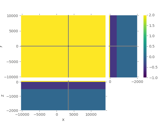
# QC
grid_1.plot_3d_slicer(
np.log10(model_1.property_x), zlim=(-2000, 100), clim=[-1, 2])
# Solve the system
efield_1 = emg3d.solve_source(model_1, source, frequency, verb=3)
:: emg3d START :: 21:49:46 :: v1.8.7

   MG-cycle       : 'F'                 sslsolver : 'bicgstab'
   semicoarsening : True [1 2 3]        tol       : 1e-06
   linerelaxation : True [4 5 6]        maxit     : 50 (3)
   nu_{i,1,c,2}   : 0, 2, 1, 2          verb      : 3
   Original grid  : 128 x  32 x  48     => 196,608 cells
   Coarsest grid  :   2 x   2 x   3     => 12 cells
   Coarsest level :   6 ;   4 ;   4

:: emg3d :: 1.2e-02; 0(1); 0:00:01
:: emg3d :: 1.4e-03; 0(2); 0:00:02
:: emg3d :: 1.8e-04; 0(3); 0:00:04
:: emg3d :: 6.6e-05; 0(4); 0:00:05
:: emg3d :: 7.9e-06; 0(5); 0:00:06
:: emg3d :: 1.2e-06; 0(6); 0:00:07
:: emg3d :: 7.8e-07; 1(6); 0:00:07

   > CONVERGED
   > Solver steps     : 1
   > MG prec. steps   : 6
   > Final rel. error : 7.844e-07

:: emg3d END   :: 21:49:53 :: runtime = 0:00:07
2nd grid, considering air resistivity for +/- x, +/- y, and +z#
See comments below the heading of the 1st grid regarding boundary.
         == GRIDDING IN X ==
Skin depth     [m] : 872 / 15915 / 15915  [corr. to `properties`]
Survey dom. DS [m] : -500 - 7500
Comp. dom. DC  [m] : -100000 - 100000
Final extent   [m] : -101682 - 108682
Cell widths    [m] : 100 / 100 / 20173  [min(DS) / max(DS) / max(DC)]
Number of cells    : 128 (80 / 48 / 0)  [Total (DS/DC/remain)]
Max stretching     : 1.000 (1.000) / 1.247  [DS (seasurface) / DC]

         == GRIDDING IN Y ==
Skin depth     [m] : 872 / 15915 / 15915  [corr. to `properties`]
Survey dom. DS [m] : 0 - 0
Comp. dom. DC  [m] : -100000 - 100000
Final extent   [m] : -102877 - 102877
Cell widths    [m] : 100 / 100 / 15539  [min(DS) / max(DS) / max(DC)]
Number of cells    : 64 (2 / 62 / 0)  [Total (DS/DC/remain)]
Max stretching     : 1.000 (1.000) / 1.177  [DS (seasurface) / DC]

         == GRIDDING IN Z ==
Skin depth     [m] : 872 / 1592 / 15915  [corr. to `properties`]
Survey dom. DS [m] : -600 - 100
Comp. dom. DC  [m] : -10600 - 99400
Final extent   [m] : -12620 - 102179
Cell widths    [m] : 100 / 100 / 19514  [min(DS) / max(DS) / max(DC)]
Number of cells    : 48 (8 / 40 / 0)  [Total (DS/DC/remain)]
Max stretching     : 1.000 (1.000) / 1.235  [DS (seasurface) / DC]
# Create corresponding model
res_2 = resistivity[0]*np.ones(grid_2.n_cells)
res_2[grid_2.cell_centers[:, 2] > -water_depth] = resistivity[1]
res_2[grid_2.cell_centers[:, 2] > 0] = resistivity[2]
model_2 = emg3d.Model(grid_2, property_x=res_2, mapping='Resistivity')

# QC
# grid_2.plot_3d_slicer(
#         np.log10(model_2.property_x), zlim=(-2000, 100), clim=[-1, 2])

# Define source and solve the system
efield_2 = emg3d.solve_source(model_2, source, frequency, verb=3)
:: emg3d START :: 21:49:53 :: v1.8.7

   MG-cycle       : 'F'                 sslsolver : 'bicgstab'
   semicoarsening : True [1 2 3]        tol       : 1e-06
   linerelaxation : True [4 5 6]        maxit     : 50 (3)
   nu_{i,1,c,2}   : 0, 2, 1, 2          verb      : 3
   Original grid  : 128 x  64 x  48     => 393,216 cells
   Coarsest grid  :   2 x   2 x   3     => 12 cells
   Coarsest level :   6 ;   5 ;   4

:: emg3d :: 1.0e-02; 0(1); 0:00:02
:: emg3d :: 1.9e-03; 0(2); 0:00:05
:: emg3d :: 5.0e-04; 0(3); 0:00:07
:: emg3d :: 6.0e-05; 0(4); 0:00:09
:: emg3d :: 1.0e-05; 0(5); 0:00:12
:: emg3d :: 3.2e-06; 0(6); 0:00:14
:: emg3d :: 2.5e-06; 1(6); 0:00:14
:: emg3d :: 2.2e-07; 1(7); 0:00:17

   > CONVERGED
   > Solver steps     : 1
   > MG prec. steps   : 7
   > Final rel. error : 2.217e-07

:: emg3d END   :: 21:50:10 :: runtime = 0:00:17
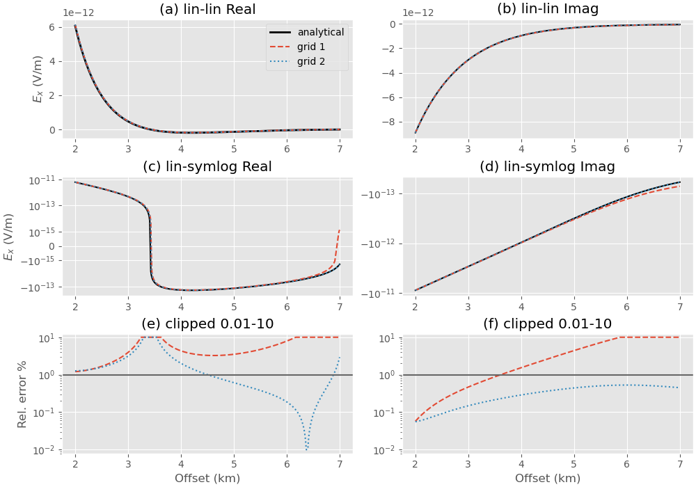
Plot receiver responses#
# Interpolate fields at receiver positions
emg_1 = efield_1.get_receiver(tuple(rec_coo))
emg_2 = efield_2.get_receiver(tuple(rec_coo))
plt.figure(figsize=(10, 7), constrained_layout=True)

# Real, log-lin
ax1 = plt.subplot(321)
plt.title('(a) lin-lin Real')
plt.plot(offsets/1e3, epm.real, 'k', lw=2, label='analytical')
plt.plot(offsets/1e3, emg_1.real, 'C0--', label='grid 1')
plt.plot(offsets/1e3, emg_2.real, 'C1:', label='grid 2')
plt.ylabel('$E_x$ (V/m)')
plt.legend()

# Real, log-symlog
ax3 = plt.subplot(323, sharex=ax1)
plt.title('(c) lin-symlog Real')
plt.plot(offsets/1e3, epm.real, 'k')
plt.plot(offsets/1e3, emg_1.real, 'C0--')
plt.plot(offsets/1e3, emg_2.real, 'C1:')
plt.ylabel('$E_x$ (V/m)')
plt.yscale('symlog', linthresh=1e-15)

# Real, error
ax5 = plt.subplot(325, sharex=ax3)
plt.title('(e) clipped 0.01-10')

# Compute the error
err_real_1 = np.clip(100*abs((epm.real-emg_1.real)/epm.real), 0.01, 10)
err_real_2 = np.clip(100*abs((epm.real-emg_2.real)/epm.real), 0.01, 10)

plt.ylabel('Rel. error %')
plt.plot(offsets/1e3, err_real_1, 'C0--')
plt.plot(offsets/1e3, err_real_2, 'C1:')
plt.axhline(1, color='.4')

plt.yscale('log')
plt.ylim([0.008, 12])
plt.xlabel('Offset (km)')

# Imaginary, log-lin
ax2 = plt.subplot(322)
plt.title('(b) lin-lin Imag')
plt.plot(offsets/1e3, epm.imag, 'k')
plt.plot(offsets/1e3, emg_1.imag, 'C0--')
plt.plot(offsets/1e3, emg_2.imag, 'C1:')

# Imaginary, log-symlog
ax4 = plt.subplot(324, sharex=ax2)
plt.title('(d) lin-symlog Imag')
plt.plot(offsets/1e3, epm.imag, 'k')
plt.plot(offsets/1e3, emg_1.imag, 'C0--')
plt.plot(offsets/1e3, emg_2.imag, 'C1:')

plt.yscale('symlog', linthresh=1e-15)

# Imaginary, error
ax6 = plt.subplot(326, sharex=ax2)
plt.title('(f) clipped 0.01-10')

# Compute error
err_imag_1 = np.clip(100*abs((epm.imag-emg_1.imag)/epm.imag), 0.01, 10)
err_imag_2 = np.clip(100*abs((epm.imag-emg_2.imag)/epm.imag), 0.01, 10)

plt.plot(offsets/1e3, err_imag_1, 'C0--')
plt.plot(offsets/1e3, err_imag_2, 'C1:')
plt.axhline(1, color='.4')

plt.yscale('log')
plt.ylim([0.008, 12])
plt.xlabel('Offset (km)')
Plot entire fields to analyze and compare#
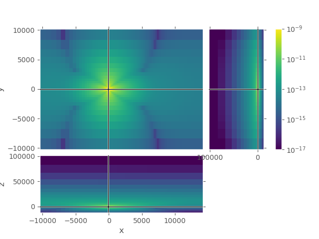
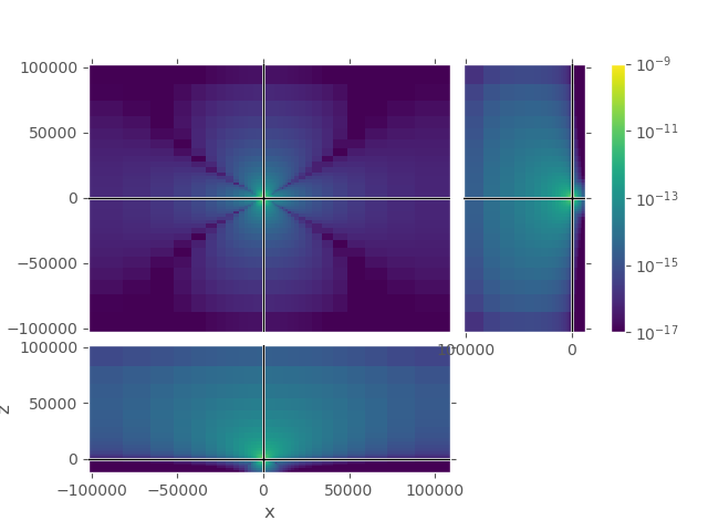
1st grid#
Upper plot shows the entire grid. One can see that the airwave attenuates to amplitudes in the order of 1e-17 at the boundary, absolutely good enough. However, the amplitudes in the horizontal directions are very high even at the boundaries \(\pm x\) and \(\pm y\).
grid_1.plot_3d_slicer(
    efield_1.fx.ravel('F'), view='abs', v_type='Ex',
    xslice=src_coo[0], yslice=src_coo[1], zslice=rec_coo[2],
    pcolor_opts={'norm': LogNorm(vmin=1e-17, vmax=1e-9)})
grid_1.plot_3d_slicer(
    efield_1.fx.ravel('F'), view='abs', v_type='Ex',
    zlim=[-5000, 1000],
    xslice=src_coo[0], yslice=src_coo[1], zslice=rec_coo[2],
    pcolor_opts={'norm': LogNorm(vmin=1e-17, vmax=1e-9)})
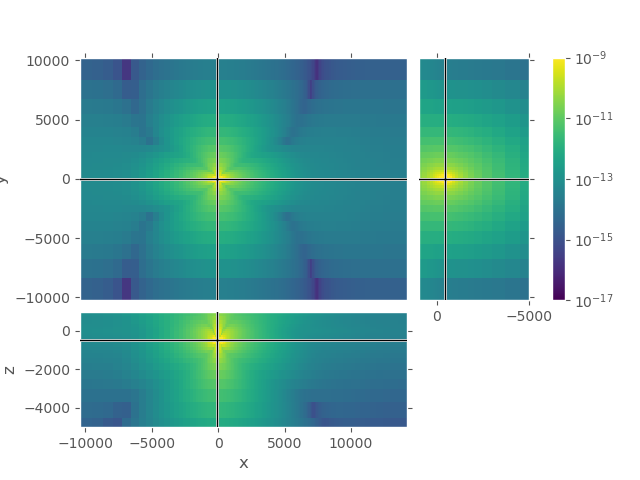
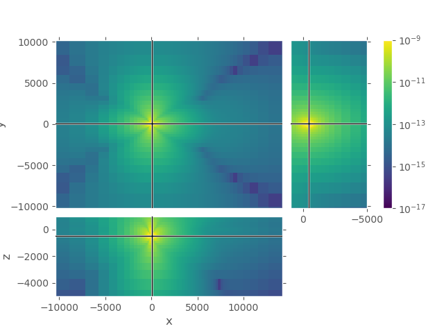
2nd grid#
Again, upper plot shows the entire grid. One can see that the field attenuated sufficiently in all directions. Lower plot shows the same cut-out as the lower plot for the first grid, our zone of interest.
grid_2.plot_3d_slicer(
    efield_2.fx.ravel('F'), view='abs', v_type='Ex',
    xslice=src_coo[0], yslice=src_coo[1], zslice=rec_coo[2],
    pcolor_opts={'norm': LogNorm(vmin=1e-17, vmax=1e-9)})
grid_2.plot_3d_slicer(
    efield_2.fx.ravel('F'), view='abs', v_type='Ex',
    xlim=[grid_1.nodes_x[0], grid_1.nodes_x[-1]],  # Same square as grid_1
    ylim=[grid_1.nodes_y[0], grid_1.nodes_y[-1]],  # Same square as grid_1
    zlim=[-5000, 1000],
    xslice=src_coo[0], yslice=src_coo[1], zslice=rec_coo[2],
    pcolor_opts={'norm': LogNorm(vmin=1e-17, vmax=1e-9)})
Total running time of the script: (0 minutes 34.081 seconds)
Estimated memory usage: 552 MB