8. Magnetic source using duality

Computing the \(E\) and \(H\) fields from a magnetic source using the duality principle.

We know that we can get the magnetic fields from the electric fields using Faraday’s law, see 6. Magnetic field due to an el. source.

However, what about computing the fields generated by a magnetic source? There are two ways we can achieve that:

• using the duality principle, which is what we do in this example, or

• creating an electric loop source, see 7. Magnetic source using an electric loop.

emg3d solves the following equation,

(1)\[ \eta \mathbf{\hat{E}} - \nabla \times \zeta^{-1} \nabla \times \mathbf{\hat{E}} = -\mathbf{\hat{J}}^e_s ,\]

where \(\eta = \sigma - \mathrm{i}\omega\varepsilon\), \(\zeta = \mathrm{i}\omega\mu\), \(\sigma\) is conductivity (S/m), \(\omega=2\pi f\) is the angular frequency (Hz), \(\mu=\mu_0\mu_\mathrm{r}\) is magnetic permeability (H/m), \(\varepsilon=\varepsilon_0\varepsilon_\mathrm{r}\) is electric permittivity (F/m), \(\mathbf{\hat{E}}\) the electric field in the frequency domain (V/m), and \(\mathbf{\hat{J}}^e_s\) source current.

This is the electric field due to an electric source. One can obtain the magnetic field due to a magnetic field by substituting

• \(\eta \leftrightarrow -\zeta\) ,

• \(\mathbf{\hat{E}} \leftrightarrow -\mathbf{\hat{H}}\) ,

• \(\mathbf{\hat{J}}^e_s \leftrightarrow \mathbf{\hat{J}}^m_s\) ,

which is called the duality principle.

Carrying out the substitution yields

(2)\[\zeta \mathbf{\hat{H}} - \nabla \times \eta^{-1} \nabla \times \mathbf{\hat{H}} = -\mathbf{\hat{J}}^m_s ,\]

which is for a magnetic dipole. Changing it for a loop source adds a term \(\mathrm{i}\omega\mu\) to the source term, resulting in

(3)\[\zeta \mathbf{\hat{H}} - \nabla \times \eta^{-1} \nabla \times \mathbf{\hat{H}} = -\mathrm{i}\omega\mu\mathbf{\hat{J}}^m_s ;\]

see Dipoles and Loops for more information.

emg3d is not ideal for the duality principle. Magnetic permeability is implemented isotropically, and discontinuities in magnetic permeabilities can lead to first-order errors in contrary to second-order errors for discontinuities in conductivity. However, we can still abuse the code and use it with the duality principle, at least for isotropic media.

The actual implemented equation in emg3d is a slightly modified version of Equation (1), using the diffusive approximation \(\varepsilon=0\),

(4)\[\mathrm{i}\omega \mu_0 \sigma \mathbf{\hat{E}} - \nabla \times \mu_r^{-1} \nabla \times \mathbf{\hat{E}} = -\mathrm{i}\omega\mu_0\mathbf{\hat{J}}_s .\]

We therefore only need to interchange \(\sigma\) with \(\mu_\mathrm{r}^{-1}\) or \(\rho\) with \(\mu_\mathrm{r}\) to get from (4) to (3).

This is what we do in this example, for an arbitrarily rotated loop in a homogeneous, isotropic fullspace. We compare the result to the semi-analytical solution of empymod. (The code empymod is an open-source code which can model CSEM responses for a layered medium including VTI electrical anisotropy, see emsig.xyz.)

import emg3d
import empymod
import numpy as np
import matplotlib.pyplot as plt

Full-space model for a rotated magnetic loop

In order to shorten the build-time of the gallery we use a coarse model. Set coarse_model = False to obtain a result of higher accuracy.

coarse_model = True

Survey and model parameters

# Receiver coordinates
if coarse_model:
    x = (np.arange(256))*20-2550
else:
    x = (np.arange(1025))*5-2560
rx = np.repeat([x, ], np.size(x), axis=0)
ry = rx.transpose()
frx, fry = rx.ravel(), ry.ravel()
rz = -400.0
azimuth = 25
elevation = 10

# Source coordinates, frequency, and strength
source = emg3d.TxElectricDipole(
    coordinates=[0, 0, -300, 10, 70],  # [x, y, z, azimuth, elevation]
    strength=np.pi,  # A
)
frequency = 0.77  # Hz

# Model parameters
h_res = 2.              # Horizontal resistivity

empymod

Note: The coordinate system of empymod is positive z down, for emg3d it is positive z up. We have to switch therefore src_z, rec_z, and elevation.

# Collect common input for empymod.
inp = {
    'src': np.r_[source.coordinates[:2], -source.coordinates[2],
                 source.coordinates[3], -source.coordinates[4]],
    'depth': [],
    'res': h_res,
    'strength': source.strength,
    'freqtime': frequency,
    'htarg': {'pts_per_dec': -1},
}

# Compute e-field
epm_e = -empymod.loop(
    rec=[frx, fry, -rz, azimuth, -elevation], mrec=False, verb=3, **inp
).reshape(np.shape(rx))

# Compute h-field
epm_h = empymod.loop(
    rec=[frx, fry, -rz, azimuth, -elevation], **inp
).reshape(np.shape(rx))

:: empymod START  ::  v2.2.0

   depth       [m] :
   res     [Ohm.m] :  2
   aniso       [-] :  1
   epermH      [-] :  1
   epermV      [-] :  1
   mpermH      [-] :  1
   mpermV      [-] :  1

>  MODEL IS A FULLSPACE
   direct field    :  Comp. in wavenumber domain
   frequency  [Hz] :  0.77
   Hankel          :  DLF (Fast Hankel Transform)
     > Filter      :  Key 201 (2009)
     > DLF type    :  Lagged Convolution
   Loop over       :  Frequencies
   Source(s)       :  1 dipole(s)
     > x       [m] :  0
     > y       [m] :  0
     > z       [m] :  300
     > azimuth [°] :  10
     > dip     [°] :  -70
   Receiver(s)     :  65536 dipole(s)
     > x       [m] :  -2550 - 2550 : 65536  [min-max; #]
     > y       [m] :  -2550 - 2550 : 65536  [min-max; #]
     > z       [m] :  400
     > azimuth [°] :  25
     > dip     [°] :  -10
   Required ab's   :  14 15 16 24 25 26 34 35 36

:: empymod END; runtime = 0:00:00.167794 :: 8 kernel call(s)


:: empymod END; runtime = 0:00:00.181631 :: 9 kernel call(s)

emg3d

if coarse_model:
    min_width_limits = 40
    stretching = [1.045, 1.045]
else:
    min_width_limits = 20
    stretching = [1.03, 1.045]

# Create stretched grid
grid = emg3d.construct_mesh(
    frequency=frequency,
    properties=h_res,
    center=source.center,
    domain=([-2500, 2500], [-2500, 2500], [-2900, 2100]),
    min_width_limits=min_width_limits,
    stretching=stretching,
    lambda_from_center=True,
    lambda_factor=0.8,
    center_on_edge=False,
)
grid

TensorMesh			884,736 cells
		MESH EXTENT		CELL WIDTH		FACTOR
dir	nC	min	max	min	max	max
x	96	-5,353.03	5,617.20	40.00	264.17	1.05
y	96	-5,353.03	5,617.20	40.00	264.17	1.05
z	96	-5,835.51	4,995.26	40.00	253.27	1.04

Abuse the parameters to take advantage of the duality principle

See text at the top. We set here \(\rho=1\) and \(\mu_\mathrm{r} = 1/\rho\) to get:

(5)\[\mathrm{i}\omega\mu_0(1-\mathrm{i}\omega\varepsilon) = \mathrm{i}\omega\mu_0+\omega^2\mu_0\varepsilon \approx \mathrm{i}\omega\mu\]

(in the diffusive regime), and

(6)\[\mu_\mathrm{r} = 1/\rho = \sigma \, .\]

# Define the model        => Set property_x = 1 and mu_r = 1./h_res
model = emg3d.Model(
    grid, property_x=1., mu_r=1./h_res, mapping='Resistivity')

# Compute the electric field
hfield = emg3d.solve_source(model, source, frequency, verb=4, plain=True)

:: emg3d START :: 21:47:59 :: v1.8.0

   MG-cycle       : 'F'                 sslsolver : False
   semicoarsening : False [0]           tol       : 1e-06
   linerelaxation : False [0]           maxit     : 50
   nu_{i,1,c,2}   : 0, 2, 1, 2          verb      : 4
   Original grid  :  96 x  96 x  96     => 884,736 cells
   Coarsest grid  :   3 x   3 x   3     => 27 cells
   Coarsest level :   5 ;   5 ;   5

   [hh:mm:ss]  rel. error                  [abs. error, last/prev]   l s

       h_
      2h_ \                            /
      4h_  \                  /\      /
      8h_   \          /\    /  \    /
     16h_    \    /\  /  \  /    \  /
     32h_     \/\/  \/    \/      \/

   [21:48:04]   3.240e-02  after   1 F-cycles   [3.094e-07, 0.032]   0 0
   [21:48:09]   2.986e-03  after   2 F-cycles   [2.851e-08, 0.092]   0 0
   [21:48:13]   3.054e-04  after   3 F-cycles   [2.916e-09, 0.102]   0 0
   [21:48:18]   3.300e-05  after   4 F-cycles   [3.151e-10, 0.108]   0 0
   [21:48:23]   3.965e-06  after   5 F-cycles   [3.786e-11, 0.120]   0 0
   [21:48:27]   8.931e-07  after   6 F-cycles   [8.529e-12, 0.225]   0 0

   > CONVERGED
   > MG cycles        : 6
   > Final rel. error : 8.931e-07

:: emg3d END   :: 21:48:27 :: runtime = 0:00:28

Plot function

def plot(epm, e3d, title, vmin, vmax):

    # Start figure.
    a_kwargs = {'cmap': "viridis", 'vmin': vmin, 'vmax': vmax,
                'shading': 'nearest'}

    e_kwargs = {'cmap': plt.cm.get_cmap("RdBu_r", 8),
                'vmin': -2, 'vmax': 2, 'shading': 'nearest'}

    fig, axs = plt.subplots(2, 3, figsize=(10, 5.5), sharex=True, sharey=True,
                            subplot_kw={'box_aspect': 1})

    ((ax1, ax2, ax3), (ax4, ax5, ax6)) = axs
    x3 = x/1000  # km

    # Plot Re(data)
    ax1.set_title(r"(a) |Re(empymod)|")
    cf0 = ax1.pcolormesh(x3, x3, np.log10(epm.real.amp()), **a_kwargs)

    ax2.set_title(r"(b) |Re(emg3d)|")
    ax2.pcolormesh(x3, x3, np.log10(e3d.real.amp()), **a_kwargs)

    ax3.set_title(r"(c) Error real part")
    rel_error = 100*np.abs((epm.real - e3d.real) / epm.real)
    cf2 = ax3.pcolormesh(x3, x3, np.log10(rel_error), **e_kwargs)

    # Plot Im(data)
    ax4.set_title(r"(d) |Im(empymod)|")
    ax4.pcolormesh(x3, x3, np.log10(epm.imag.amp()), **a_kwargs)

    ax5.set_title(r"(e) |Im(emg3d)|")
    ax5.pcolormesh(x3, x3, np.log10(e3d.imag.amp()), **a_kwargs)

    ax6.set_title(r"(f) Error imaginary part")
    rel_error = 100*np.abs((epm.imag - e3d.imag) / epm.imag)
    ax6.pcolormesh(x3, x3, np.log10(rel_error), **e_kwargs)

    # Colorbars
    unit = "(V/m)" if "E" in title else "(A/m)"
    fig.colorbar(cf0, ax=axs[0, :], label=r"$\log_{10}$ Amplitude "+unit)
    cbar = fig.colorbar(cf2, ax=axs[1, :], label=r"Relative Error")
    cbar.set_ticks([-2, -1, 0, 1, 2])
    cbar.ax.set_yticklabels([r"$0.01\,\%$", r"$0.1\,\%$", r"$1\,\%$",
                             r"$10\,\%$", r"$100\,\%$"])

    ax1.set_xlim(min(x3), max(x3))
    ax1.set_ylim(min(x3), max(x3))

    # Axis label
    fig.text(0.4, 0.05, "Inline Offset (km)", fontsize=14)
    fig.text(0.05, 0.3, "Crossline Offset (km)", rotation=90, fontsize=14)
    fig.suptitle(title, y=1, fontsize=20)

    print(f"- Source: {source}")
    print(f"- Frequency: {frequency} Hz")
    rtype = "Electric" if "E" in title else "Magnetic"
    print(f"- {rtype} receivers: z={rz} m; θ={azimuth}°, φ={elevation}°")

    fig.show()

Compare the magnetic field generated from the magnetic source

e3d_h = hfield.get_receiver((rx, ry, rz, azimuth, elevation))
plot(epm_h, e3d_h, r'Diffusive Fullspace $H$', vmin=-15, vmax=-8)

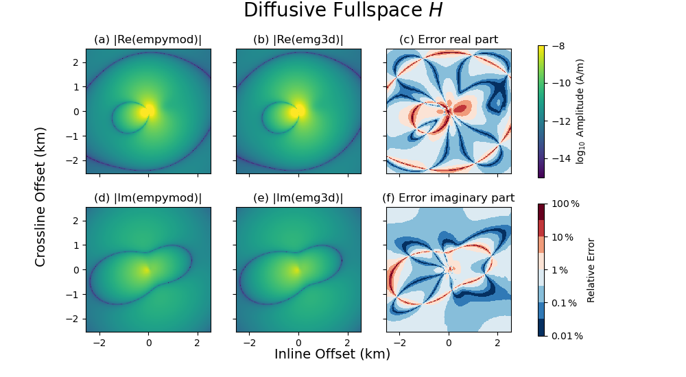
- Source: TxElectricDipole: 3.1 A;
    center={0.0; 0.0; -300.0} m; θ=10.0°, φ=70.0°; l=1.0 m
- Frequency: 0.77 Hz
- Magnetic receivers: z=-400.0 m; θ=25°, φ=10°

Compare the electric field generated from the magnetic source

get_magnetic_field gets the \(H\)-field from the \(E\)-field with Faraday’s law,

(7)\[\nabla \times \mathbf{E} = \rm{i}\omega \mathbf{B} = \rm{i}\omega\mu\mathbf{H}\, .\]

Using the substitutions introduced in the beginning, and using the same function but to get the \(E\)-field from the \(H\)-field, we have to multiply the result by

(8)\[\rm{i}\omega\mu\, .\]

Compute electric field \(E\) from the magnetic field

efield = emg3d.get_magnetic_field(model, hfield)
efield.field *= efield.smu0

e3d_e = efield.get_receiver((rx, ry, rz, azimuth, elevation))
plot(epm_e, e3d_e, r'Diffusive Fullspace $E$', vmin=-17, vmax=-10)

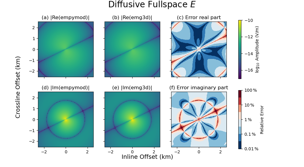
- Source: TxElectricDipole: 3.1 A;
    center={0.0; 0.0; -300.0} m; θ=10.0°, φ=70.0°; l=1.0 m
- Frequency: 0.77 Hz
- Electric receivers: z=-400.0 m; θ=25°, φ=10°

emg3d.Report()

Wed Aug 31 21:48:31 2022 CEST
OS	Linux	CPU(s)	4	Machine	x86_64
Architecture	64bit	RAM	15.5 GiB	Environment	Python
File system	ext4
Python 3.9.12 | packaged by conda-forge | (main, Mar 24 2022, 23:22:55) [GCC 10.3.0]
numpy	1.22.4	scipy	1.9.0	numba	0.55.2
emg3d	1.8.0	empymod	2.2.0	xarray	2022.6.0
discretize	0.8.2	h5py	3.7.0	matplotlib	3.4.3
tqdm	4.64.0	IPython	8.4.0
Intel(R) oneAPI Math Kernel Library Version 2022.0-Product Build 20211112 for Intel(R) 64 architecture applications

Estimated memory usage: 174 MB