10. Layered

Since v1.8.0 there exists the possibility to use locally approximated, layered models together with empymod to compute responses and the gradient instead of the 3D model with emg3d.

Here we look at this possibility by reproducing the example 04. Gradient of the misfit function. (Please note, however, that the layered option does not only work for the gradient, but also for pure forward modelling.)

For this example we use the resistivity model created in the example GemPy-II: Perth Basin, together with the survey created in 03. Simulation.

Limitations

The limitations of the layered modelling are:

• Only point and dipole sources.

• Only isotropic and VTI models.

Also, using the layered modelling has a few other implications, e.g.:

• There are no {e;h}fields, only the fields at receiver locations.

• gridding, most of gridding_opts, solver_opts, receiver_interpolation, and file_dir have no effect.

• The attribute emg3d.simulations.Simulation.jvec is not implemented.

Some considerations about speed

If you are concerned about speed take into account that using layered computations changes the things one has to consider.

• “Regular” 3D:

  • Linear with number of source-frequency pairs; parallelized over it.

  • Depends on gridding options; linear in number of cells.

  • Extra receivers at almost no extra cost.

• “Layered” 1D:

  • Linear with number of source-receiver pairs; parallelized over sources; serial over receivers.

  • Only for the gradient: depends linearly on the number of layers in the provided model.

  • Extra frequencies at little extra cost.

import os
import pooch
import emg3d
import numpy as np
import matplotlib.pyplot as plt
from matplotlib.colors import LogNorm, SymLogNorm

# Adjust this path to a folder of your choice.
data_path = os.path.join('..', 'download', '')

Load survey, data, and model

First we load the model, survey, and accompanying data as obtained in the examples GemPy-II: Perth Basin and 03. Simulation (check these examples for more information).

isurvey = (
    'GemPy-II-survey-A.h5',
    '5f2ed0b959a4f80f5378a071e6f729c6b7446898be7689ddc9bbd100a8f5bce7',
)
imodel = (
    'GemPy-II.h5',
    'ea8c23be80522d3ca8f36742c93758370df89188816f50cb4e1b2a6a3012d659',
)

# Download model and survey.
for data in [isurvey, imodel]:
    pooch.retrieve(
        'https://raw.github.com/emsig/data/2021-05-21/emg3d/surveys/'+data[0],
        data[1], fname=data[0], path=data_path,
    )

# Load them.
survey = emg3d.load(os.path.join(data_path, isurvey[0]))['survey']
true_model = emg3d.load(os.path.join(data_path, imodel[0]))['model']
grid = true_model.grid

Data loaded from «/home/dtr/3-GitHub/emsig/emg3d-gallery/examples/download/GemPy-II-survey-A.h5»
[emg3d v0.17.1.dev22+ge23c468 (format 1.0) on 2021-04-14T22:24:03.229285].
Data loaded from «/home/dtr/3-GitHub/emsig/emg3d-gallery/examples/download/GemPy-II.h5»
[emg3d v1.0.0rc3.dev5+g0cd9e09 (format 1.0) on 2021-05-21T18:40:16.721968].

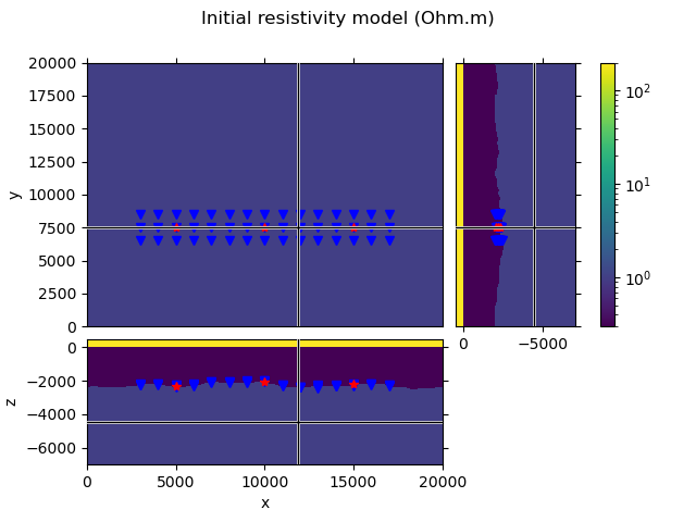
Create an initial model

To create an initial model we take the true model, but set all subsurface resistivities to 1 Ohm.m. So we are left with a homogeneous three-layer model air-seawater-subsurface, which includes the topography of the seafloor.

# Overwrite all subsurface resistivity values with 1.0
model = true_model.copy()
res = model.property_x
subsurface = (res > 0.5) & (res < 1000)
res[subsurface] = 1.0
model.property_x = res

# QC the initial model and the survey.
popts = {'norm': LogNorm(vmin=0.3, vmax=200)}
grid.plot_3d_slicer(
    model.property_x, xslice=12000, yslice=7500, pcolor_opts=popts
)

# Plot survey in figure above
fig = plt.gcf()
fig.suptitle('Initial resistivity model (Ohm.m)')
axs = fig.get_children()
rec_coords = survey.receiver_coordinates()
src_coords = survey.source_coordinates()
axs[1].plot(rec_coords[0], rec_coords[1], 'bv')
axs[2].plot(rec_coords[0], rec_coords[2], 'bv')
axs[3].plot(rec_coords[2], rec_coords[1], 'bv')
axs[1].plot(src_coords[0], src_coords[1], 'r*')
axs[2].plot(src_coords[0], src_coords[2], 'r*')
axs[3].plot(src_coords[2], src_coords[1], 'r*')
plt.show()

Options for layered computation

If layered=True, one can provide a layered_opts-dict to a simulation. For more information about this see towards the end of this example. The simulation uses some defaults values, if they are not provided. By default a local 1D model is generated by creating a right elliptic cylinder around source and receiver position, and average the values for each layer within this cylinder.

You can read more about the local extraction and the ellipse options in the functions emg3d.models.Model.extract_1d and emg3d.maps.ellipse_indices().

Note that using layered computations means that we do not have to provide any gridding options, as there is no gridding happening.

Create the Simulation

simulation = emg3d.simulations.Simulation(
    name="Initial Model",
    survey=survey,
    model=model,
    max_workers=4,
    layered=True,            # Set layered to True!
    # layered_opts=...,      # Parameters for the local 1D extractions.
)

# Let's QC our Simulation instance
simulation

Simulation «Initial Model»

• Survey «GemPy-II Survey A»: 3 sources; 45 receivers; 2 frequencies
• Model: resistivity; isotropic; 100 x 100 x 102 (1,020,000)
• Gridding: layered computation using method 'cylinder'; radius: 711.76; factor: 1.20; minor: 0.80

The simulation indicates that it uses layered computations with the method 'cylinder' and certain ellipse-parameters.

Compute Gradient

Let’s compute the gradient (with layered=True!).

grad = simulation.gradient

Compute empymod            0/3  [00:00]
Compute empymod ###3       1/3  [00:01]
Compute empymod ########## 3/3  [00:01]

Compute empymod            0/3  [00:00]
Compute empymod ###3       1/3  [00:32]
Compute empymod ######6    2/3  [00:36]
Compute empymod ########## 3/3  [00:36]

QC Gradient

# Set the gradient of air and water to NaN.
# This will eventually move directly into emgd3 (active and inactive cells).
grad[~subsurface] = np.nan


# Plot the gradient
grid.plot_3d_slicer(
    grad.ravel('F'), xslice=12000, yslice=7500, zslice=-4000,
    pcolor_opts={
        'cmap': 'RdBu_r',
        'norm': SymLogNorm(linthresh=1e-2, base=10, vmin=-1e1, vmax=1e1)
    }
)

# Add survey
fig = plt.gcf()
fig.suptitle('Gradient of the misfit function')
axs = fig.get_children()
axs[1].plot(rec_coords[0], rec_coords[1], 'bv')
axs[2].plot(rec_coords[0], rec_coords[2], 'bv')
axs[3].plot(rec_coords[2], rec_coords[1], 'bv')
axs[1].plot(src_coords[0], src_coords[1], 'r*')
axs[2].plot(src_coords[0], src_coords[2], 'r*')
axs[3].plot(src_coords[2], src_coords[1], 'r*')
plt.show()

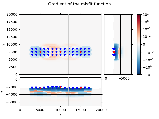
Even though we use layered (1D) models, the gradient looks three dimensional. This is because each source-receiver pair has its own cylinder, from which it generates a 1D model. The resulting gradient is then projected back to the same cylinder. This yields, summing up all source-receiver pairs, a three-dimensional gradient.

Note that this gradient is obtained using the finite-difference method, by perturbing each layer by a tiny bit. This is in contrast to the gradient obtained with emg3d, where the adjoint-state method is used.

Compare this gradient to the adjoint-state gradient, obtained by true 3D computations, in example 04. Gradient of the misfit function.

A few words about the 1D model extraction

There are five possible methods: cylinder, prism, midpoint, source, and receiver. However, in reality they reduce to really two different possibility:

• 'midpoint': If midpoint is chosen, the selected 1D model is simply the column midway between the two provided points, usually source and receiver. 'source' and 'receiver' only differ in that both points are set to source or receiver, respectively, meaning that the column at source or receiver location is selected.

• 'cylinder': If cylinder is chosen, a right elliptic cylinder around the two points is selected. How the ellipse is selected depends on a few other parameters, see functions emg3d.models.Model.extract_1d and emg3d.maps.ellipse_indices(). The only difference for 'prism' is that it uses the rectangular, coordinate-system aligned envelope of the ellipse.

The default values are: method='cylinder'. The corresponding default values of the ellipse-options are factor=1.2, minor=0.8, and radius is set to one skin depth using the lowest frequency and the lowest conductivity value in the lowest layer in vertical direction.

Let’s look at the default value the simulation has chosen in this case:

lopts = simulation.layered_opts
lopts

{'method': 'cylinder', 'ellipse': {'radius': 711.762543223444, 'factor': 1.2, 'minor': 0.8}}

So we see that it chose the default method 'cylinder', the default values factor=1.2 and minor=0.8, and the radius is set to roughly 712 m.

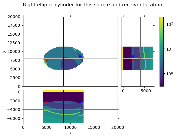
We select now one source and one receiver, to QC how the selected cylinder looks like.

src = survey.sources['TxED-1']
rec = survey.receivers['RxEP-30']

layered, imat = true_model.extract_1d(
    lopts['method'], src.center[:2], rec.center[:2], lopts['ellipse'],
    return_imat=True
)

values = true_model.property_x.copy()
values[~np.array(imat, dtype=bool), :] = np.nan

xy = (src.center[:2] + rec.center[:2])/2
grid.plot_3d_slicer(
    values, xslice=xy[0], yslice=xy[1], zslice=-4000, pcolor_opts=popts
)

fig = plt.gcf()
fig.suptitle('Right elliptic cylinder for this source and receiver location')
axs = fig.get_children()

axs[1].plot(rec.center[0], rec.center[1], 'bv')
axs[1].plot(src.center[0], src.center[1], 'r*')
axs[2].plot(rec.center[0], rec.center[2], 'bv')
axs[3].plot(rec.center[2], rec.center[1], 'bv')
axs[2].plot(src.center[0], src.center[2], 'r*')
axs[3].plot(src.center[2], src.center[1], 'r*')

plt.show()

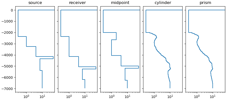
We can compare the five different methods, and see what 1D models they extract from the 3D model.

fig, axs = plt.subplots(
    1, 5, figsize=(9, 4), sharex=True, sharey=True, constrained_layout=True
)
axs = axs.ravel()

pdepth = np.repeat(true_model.grid.nodes_z[1:-1], 2)

ellipse = lopts['ellipse']
methods = ['source', 'receiver', 'midpoint', 'cylinder', 'prism']
for i, method in enumerate(methods):

    axs[i].set_title(method)

    p0 = src.center[:2]
    p1 = rec.center[:2]

    if method == 'source':
        p1 = p0
        method = 'midpoint'
    elif method == 'receiver':
        p0 = p1
        method = 'midpoint'

    oned = true_model.extract_1d(method, p0, p1, ellipse)

    res = np.repeat(oned.property_x, 2)[1:-1]

    axs[i].plot(res, pdepth)

axs[0].set_xscale('log')
axs[0].set_xlim([0.2, 60])
plt.show()

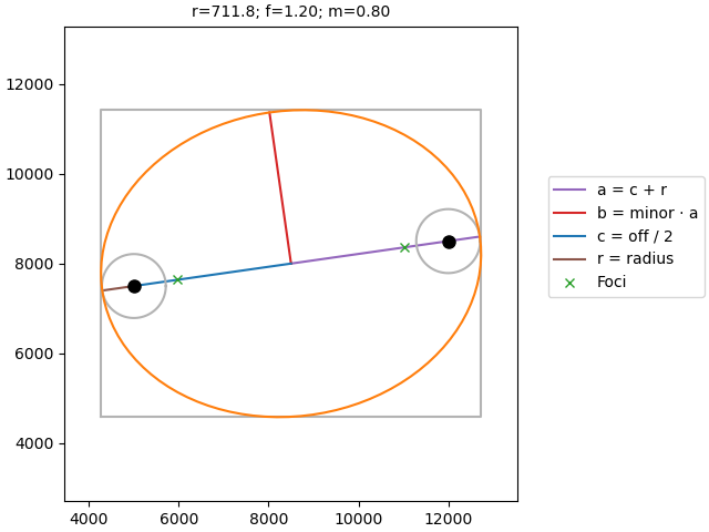
Ellipse

As mentioned before, the ellipse is selected using the function emg3d.maps.ellipse_indices(). The documentation of that function contains a lot of useful information about it. However, here is a function that illustrates the ellipse with all its parameters.

def plot_ellipse(ax, p0, p1, radius, factor=1.0, minor=1.0, check_foci=True):
    """Plot annotated explanation of emg3d.maps.ellipse_ind()."""

    # Cast input points to numpy arrays.
    p0, p1 = np.array(p0), np.array(p1)

    # Center coordinates
    cx, cy = (p0 + p1) / 2

    # Adjacent and opposite sides
    dx, dy = (p1 - p0) / 2

    # c: linear eccentricity
    dxy = np.linalg.norm([dx, dy])

    # a: semi-major axis
    major = max(dxy * factor, dxy + radius)

    # b: semi-minor axis
    minor = max(minor * major, radius)
    if check_foci:
        minor = max(minor, np.sqrt(abs(major**2 - dxy**2)))

    # Distance to foci
    df = np.sqrt(major**2 - minor**2)

    # Take care of division by zero
    if dy == 0.0:
        cos, sin = 1.0, 0.0
    else:
        cos, sin = dx/dxy, dy/dxy

    # Parametrized ellipse
    t = np.linspace(0, 2*np.pi, 101)
    cost, sint = np.cos(t), np.sin(t)
    x = cx + major*cos*cost - minor*sin*sint
    y = cy + major*sin*cost + minor*cos*sint

    # Verteces
    vr = [cx + major*cos, cy + major*sin]
    vl = [cx - major*cos, cy - major*sin]

    # Upper co-vertex
    vu = [cx - minor*sin, cy + minor*cos]

    # Foci
    fr = [cx + df*cos, cy + df*sin]
    fl = [cx - df*cos, cy - df*sin]

    # PLOTTING

    # Title with radius and _actual_ minor factor.
    ax.set_title(f"r={radius:.1f}; "
                 f"f={factor:.2f}; "
                 f"m={1.0 if major == 0.0 else minor/major:.2f}", fontsize=10)

    # Draw a, b, c, and r
    ax.plot([cx, vr[0]], [cy, vr[1]], 'C4', label=r'a = c + r')
    ax.plot([cx, vu[0]], [cy, vu[1]], 'C3', label=r'b = minor · a')
    ax.plot([p0[0], cx], [p0[1], cy], 'C0', label=r'c = off / 2')
    ax.plot([vl[0], p0[0]], [vl[1], p0[1]], 'C5', label=r'r = radius')

    # Draw the two points and their circles with radius
    for p in [p0, p1]:
        ax.plot(*p, 'o', c='k', ms=8)
        ax.plot(p[0] + radius*cost, p[1] + radius*sint, '.7')

    # Draw the foci
    ax.plot([fr[0], fl[0]], [fr[1], fl[1]], 'C2x', label='Foci')

    # Draw the envelopping square
    ax.plot([x.min(), x.max(), x.max(), x.min(), x.min()],
            [y.min(), y.min(), y.max(), y.max(), y.min()], '.7')

    # Draw the ellipse
    ax.plot(x, y, 'C1')

    # Ensure square axes
    ax.axis('equal')

Here the annotation for the above selection. However, you can use this function to test the influence of the different parameters.

fig, ax = plt.subplots(constrained_layout=True)
plot_ellipse(
    ax,
    p0=src.center[:2],
    p1=rec.center[:2],
    radius=lopts['ellipse']['radius'],
    factor=lopts['ellipse']['factor'],
    minor=lopts['ellipse']['minor'],
)
ax.legend(bbox_to_anchor=(1.05, 0.7))
plt.show()

emg3d.Report()

Wed Aug 31 22:03:18 2022 CEST
OS	Linux	CPU(s)	4	Machine	x86_64
Architecture	64bit	RAM	15.5 GiB	Environment	Python
File system	ext4
Python 3.9.12 | packaged by conda-forge | (main, Mar 24 2022, 23:22:55) [GCC 10.3.0]
numpy	1.22.4	scipy	1.9.0	numba	0.55.2
emg3d	1.8.0	empymod	2.2.0	xarray	2022.6.0
discretize	0.8.2	h5py	3.7.0	matplotlib	3.4.3
tqdm	4.64.0	IPython	8.4.0
Intel(R) oneAPI Math Kernel Library Version 2022.0-Product Build 20211112 for Intel(R) 64 architecture applications

Estimated memory usage: 165 MB