02. Model property mapping

Physical rock properties (and their units) can be a tricky thing. And emg3d is no difference in this respect. It was first developed for oil and gas, having resistive bodies in mind. You will therefore find that the documentation often talks about resistivity (Ohm.m). However, internally the computation is carried out in conductivities (S/m), so resistivities are converted into conductivities internally. For the simple forward model this is not a big issue, as the output is simply the electromagnetic field. However, moving over to optimization makes things more complicated, as the gradient of the misfit function, for instance, depends on the parametrization.

Since emg3d v0.12.0 it is therefore possible to define a emg3d.models.Model in different ways, thanks to different maps, defined with the parameter mapping. Currently implemented are six different maps:

• 'Resistivity': \(\rho\) (Ohm.m), the default;

• 'LgResistivity': \(\log_{10}(\rho)\);

• 'LnResistivity': \(\log_e(\rho)\);

• 'Conductivity': \(\sigma\) (S/m);

• 'LgConductivity': \(\log_{10}(\sigma)\);

• 'LnConductivity': \(\log_e(\sigma)\).

We take here the model from 05. Total vs primary/secondary field and map it once as 'LgResistivity' and once as 'LgConductivity', and verify that the resulting electric field is the same.

import emg3d
import numpy as np
import matplotlib.pyplot as plt
plt.style.use('bmh')

Survey

src = [0, 0, -1950, 0, 0]   # x-dir. source at the origin, 50 m above seafloor
off = np.arange(5, 81)*100  # Offsets
rec = [off, off*0, -2000]   # In-line receivers on the seafloor
res = [0.3, 1]              # 1D resistivities (Ohm.m): [water, background]
freq = 1.0                  # Frequency (Hz)

Mesh

We create quite a coarse grid (100 m minimum cell width), to have reasonable fast computation times.

grid = emg3d.construct_mesh(
        frequency=freq,
        min_width_limits=100.0,
        properties=[res[0], res[1], res[1], res[0]],
        center=(src[0], src[1], -2000),
        domain=([-100, 8100], [-500, 500], [-3500, -1500]),
        center_on_edge=True,
        verb=0,
)
grid

TensorMesh			73,728 cells
		MESH EXTENT		CELL WIDTH		FACTOR
dir	nC	min	max	min	max	max
x	96	-3,303.39	11,303.39	100.00	996.95	1.39
y	24	-3,703.39	3,703.39	100.00	996.95	1.39
z	32	-7,512.73	240.89	100.00	1,344.36	1.45

Define resistivities

# Layered_background
res_x = np.ones(grid.n_cells)*res[0]            # Water resistivity
res_x[grid.cell_centers[:, 2] < -2000] = res[1]  # Background resistivity

# Include the target
xx = (grid.cell_centers[:, 0] >= 0) & (grid.cell_centers[:, 0] <= 6000)
yy = abs(grid.cell_centers[:, 1]) <= 500
zz = (grid.cell_centers[:, 2] > -3500)*(grid.cell_centers[:, 2] < -3000)

res_x[xx*yy*zz] = 100.  # Target resistivity

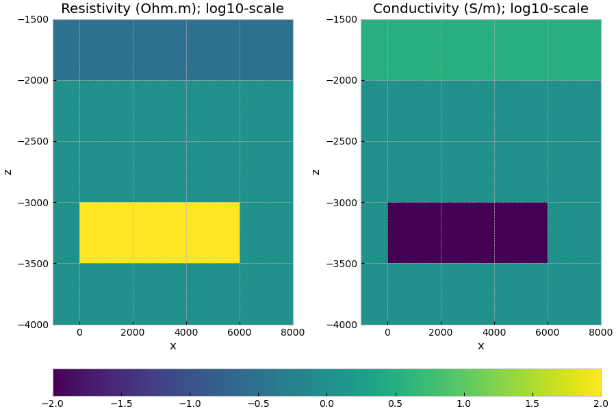
Create LgResistivity and LgConductivity models

# Create log10-res model
model_lg_res = emg3d.Model(
        grid, property_x=np.log10(res_x), mapping='LgResistivity')

# Create log10-con model
model_lg_con = emg3d.Model(
        grid, property_x=np.log10(1/res_x), mapping='LgConductivity')

# Plot the models
fig, axs = plt.subplots(figsize=(9, 6), nrows=1, ncols=2)

# log10-res
f0 = grid.plot_slice(model_lg_res.property_x, v_type='CC',
                     normal='Y', ax=axs[0], clim=[-2, 2])
axs[0].set_title(r'Resistivity (Ohm.m); $\log_{10}$-scale')
axs[0].set_xlim([-1000, 8000])
axs[0].set_ylim([-4000, -1500])

# log10-con
f1 = grid.plot_slice(model_lg_con.property_x, v_type='CC',
                     normal='Y', ax=axs[1], clim=[-2, 2])
axs[1].set_title(r'Conductivity (S/m); $\log_{10}$-scale')
axs[1].set_xlim([-1000, 8000])
axs[1].set_ylim([-4000, -1500])

plt.tight_layout()
fig.colorbar(f0[0], ax=axs, orientation='horizontal', fraction=0.05)
plt.show()

Compute electric fields

source = emg3d.TxElectricDipole(coordinates=src)
solver_opts = {
    'source': source,
    'frequency': freq,
    'verb': 1,
}

efield_lg_res = emg3d.solve_source(model_lg_res, **solver_opts)
efield_lg_con = emg3d.solve_source(model_lg_con, **solver_opts)

# Extract responses at receiver locations.
rec_lg_res = efield_lg_res.get_receiver((*rec, 0, 0))
rec_lg_con = efield_lg_con.get_receiver((*rec, 0, 0))

:: emg3d :: 8.9e-07; 1(4); 0:00:05; CONVERGED
:: emg3d :: 8.9e-07; 1(4); 0:00:05; CONVERGED

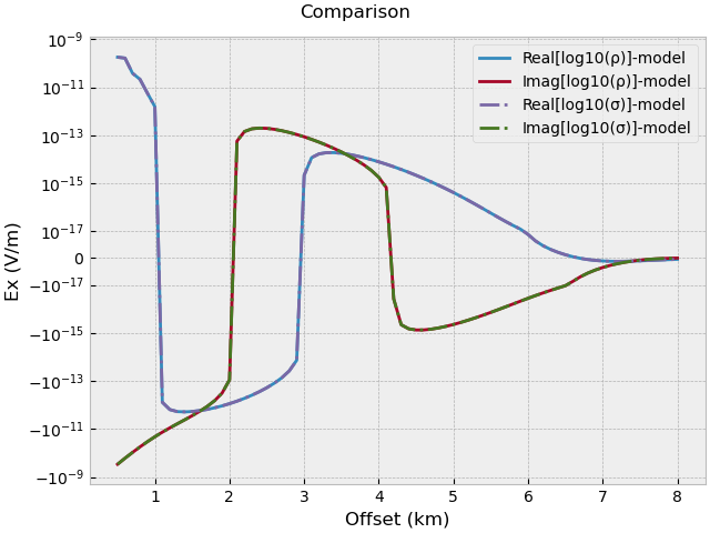
Compare the two results

plt.figure()
plt.title('Comparison')

# Log_10(resistivity)-model.
plt.plot(off/1e3, rec_lg_res.real, 'C0',
         label=r'$\Re[\log_{10}(\rho)]$-model')
plt.plot(off/1e3, rec_lg_res.imag, 'C1-',
         label=r'$\Im[\log_{10}(\rho)]$-model')

# Log_10(conductivity)-model.
plt.plot(off/1e3, rec_lg_con.real, 'C2-.',
         label=r'$\Re[\log_{10}(\sigma)]$-model')
plt.plot(off/1e3, rec_lg_con.imag, 'C3-.',
         label=r'$\Im[\log_{10}(\sigma)]$-model')

plt.xlabel('Offset (km)')
plt.ylabel('$E_x$ (V/m)')
plt.yscale('symlog', linthresh=1e-17)
plt.legend()

plt.tight_layout()
plt.show()

emg3d.Report()

Wed Aug 31 21:25:16 2022 CEST
OS	Linux	CPU(s)	4	Machine	x86_64
Architecture	64bit	RAM	15.5 GiB	Environment	Python
File system	ext4
Python 3.9.12 | packaged by conda-forge | (main, Mar 24 2022, 23:22:55) [GCC 10.3.0]
numpy	1.22.4	scipy	1.9.0	numba	0.55.2
emg3d	1.8.0	empymod	2.2.0	xarray	2022.6.0
discretize	0.8.2	h5py	3.7.0	matplotlib	3.4.3
tqdm	4.64.0	IPython	8.4.0
Intel(R) oneAPI Math Kernel Library Version 2022.0-Product Build 20211112 for Intel(R) 64 architecture applications

Estimated memory usage: 45 MB