Note
Go to the end to download the full example code.
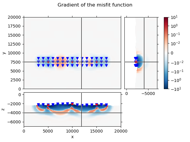
04. Gradient of the misfit function#
A basic example how to use the emg3d.simulations.Simulation.gradient
routine to compute the adjoint-state gradient of the misfit function. Here we
just show its usage.
For this example we use the survey and data as obtained in the example 03. Simulation.
import os
import pooch
import emg3d
import numpy as np
import matplotlib.pyplot as plt
from matplotlib.colors import LogNorm, SymLogNorm


# Adjust this path to a folder of your choice.
data_path = os.path.join('..', 'download', '')
Load survey and data#
First we load the survey and accompanying data as obtained in the example 03. Simulation.
Data loaded from «/home/dtr/Codes/emsig/emg3d-gallery/examples/download/GemPy-II-survey-A.h5»
[emg3d v0.17.1.dev22+ge23c468 (format 1.0) on 2021-04-14T22:24:03.229285].
We can see that the survey consists of three sources, 45 receivers, and two frequencies.
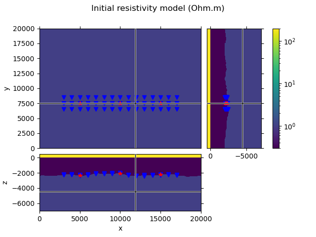
Create an initial model#
To create an initial model we load the true model, but set all subsurface resistivities to 1 Ohm.m. So we are left with a homogeneous three-layer model air-seawater-subsurface, which includes the topography of the seafloor.
# Load true model
fname = "GemPy-II.h5"
pooch.retrieve(
    'https://raw.github.com/emsig/data/2021-05-21/emg3d/models/'+fname,
    'ea8c23be80522d3ca8f36742c93758370df89188816f50cb4e1b2a6a3012d659',
    fname=fname,
    path=data_path,
)
model = emg3d.load(data_path + fname)['model']
grid = model.grid
Data loaded from «/home/dtr/Codes/emsig/emg3d-gallery/examples/download/GemPy-II.h5»
[emg3d v1.0.0rc3.dev5+g0cd9e09 (format 1.0) on 2021-05-21T18:40:16.721968].
# Overwrite all subsurface resistivity values with 1.0
res = model.property_x
subsurface = (res > 0.5) & (res < 1000)
res[subsurface] = 1.0
model.property_x = res

# QC the initial model and the survey.
grid.plot_3d_slicer(model.property_x, xslice=12000, yslice=7500,
                    pcolor_opts={'norm': LogNorm(vmin=0.3, vmax=200)})

# Plot survey in figure above
fig = plt.gcf()
fig.suptitle('Initial resistivity model (Ohm.m)')
axs = fig.get_children()
rec_coords = survey.receiver_coordinates()
src_coords = survey.source_coordinates()
axs[1].plot(rec_coords[0], rec_coords[1], 'bv')
axs[2].plot(rec_coords[0], rec_coords[2], 'bv')
axs[3].plot(rec_coords[2], rec_coords[1], 'bv')
axs[1].plot(src_coords[0], src_coords[1], 'r*')
axs[2].plot(src_coords[0], src_coords[2], 'r*')
axs[3].plot(src_coords[2], src_coords[1], 'r*')
Options for automatic gridding#
gridding_opts = {
    'center': (src_coords[0][1], src_coords[1][1], -2200),
    'properties': [0.3, 10, 1, 0.3],
    'domain': (
        [rec_coords[0].min()-100, rec_coords[0].max()+100],
        [rec_coords[1].min()-100, rec_coords[1].max()+100],
        [-5500, -2000]
    ),
    'min_width_limits': (100, 100, 50),
    'stretching': (None, None, [1.05, 1.5]),
    'center_on_edge': False,
}
Create the Simulation#
simulation = emg3d.simulations.Simulation(
    name="Initial Model",    # A name for this simulation
    survey=survey,           # Our survey instance
    model=model,             # The model
    gridding='both',         # Src- and freq-dependent grids
    max_workers=4,           # How many parallel jobs
    # solver_opts=...,       # Any parameter to pass to emg3d.solve
    gridding_opts=gridding_opts,
    receiver_interpolation='linear',  # For proper adjoint-state gradient
)

# Let's QC our Simulation instance
simulation
Compute Gradient#
Compute efields            0/6  [00:00]
Compute efields █▋         1/6  [00:23]
Compute efields █████      3/6  [00:23]
Compute efields ████████▎  5/6  [00:35]
Compute efields ██████████ 6/6  [00:35]

Back-propagate            0/6  [00:00]
Back-propagate █▋         1/6  [00:23]
Back-propagate █████      3/6  [00:23]
Back-propagate ████████▎  5/6  [00:34]
Back-propagate ██████████ 6/6  [00:34]
QC Gradient#
# Set the gradient of air and water to NaN.
# This will eventually move directly into emgd3 (active and inactive cells).
grad[~subsurface] = np.nan


# Plot the gradient
grid.plot_3d_slicer(
        grad.ravel('F'), xslice=12000, yslice=7500, zslice=-4000,
        pcolor_opts={'cmap': 'RdBu_r',
                     'norm': SymLogNorm(
                         linthresh=1e-2, base=10, vmin=-1e1, vmax=1e1)}
        )

# Add survey
fig = plt.gcf()
fig.suptitle('Gradient of the misfit function')
axs = fig.get_children()
axs[1].plot(rec_coords[0], rec_coords[1], 'bv')
axs[2].plot(rec_coords[0], rec_coords[2], 'bv')
axs[3].plot(rec_coords[2], rec_coords[1], 'bv')
axs[1].plot(src_coords[0], src_coords[1], 'r*')
axs[2].plot(src_coords[0], src_coords[2], 'r*')
axs[3].plot(src_coords[2], src_coords[1], 'r*')
Total running time of the script: (1 minutes 14.876 seconds)
Estimated memory usage: 836 MB