Note
Go to the end to download the full example code.
5. empymod: 1D VTI Laplace-domain#
1D VTI comparison between emg3d and empymod in the Laplace domain.
The code empymod is an open-source code which can model CSEM responses for
a layered medium including VTI electrical anisotropy, see emsig.xyz.
Content:
Full-space VTI model for a finite length, finite strength, rotated bipole.
Layered model for a deep water model with a point dipole source.
Both codes, empymod and emg3d, are able to compute the EM response in
the Laplace domain, by using a real value \(s\) instead of the complex
value \(\mathrm{i}\omega=2\mathrm{i}\pi f\). To compute the response in
the Laplace domain in the two codes you have to provide negative values for the
freq-parameter, which are then considered s-value.
import emg3d
import empymod
import numpy as np
import matplotlib.pyplot as plt
1. Full-space VTI model for a finite length, finite strength, rotated bipole#
In order to shorten the build-time of the gallery we use a coarse model.
Set coarse_model = False to obtain a result of higher accuracy.
coarse_model = True
Survey and model parameters#
# Receiver coordinates
if coarse_model:
    x = (np.arange(256))*20-2550
else:
    x = (np.arange(1025))*5-2560
rx = np.repeat([x, ], np.size(x), axis=0)
ry = rx.transpose()
frx, fry = rx.ravel(), ry.ravel()
rz = -400.0
azimuth = 33
elevation = 18

# Source coordinates, frequency, and strength
source = emg3d.TxElectricDipole(
    coordinates=[-50, 50, -30, 30, -320., -280.],  # [x1, x2, y1, y2, z1, z2]
    strength=3.1,  # A
)
sval = -7  # Laplace value

# Model parameters
h_res = 1.              # Horizontal resistivity
aniso = np.sqrt(2.)     # Anisotropy
v_res = h_res*aniso**2  # Vertical resistivity
1.a Regular VTI case#
empymod#
Note: The coordinate system of empymod is positive z down, for emg3d it is positive z up. We have to switch therefore src_z, rec_z, and elevation.
# Compute
epm = empymod.bipole(
    src=np.r_[source.coordinates[:4], -source.coordinates[4:]],
    depth=[],
    res=h_res,
    aniso=aniso,
    strength=source.strength,
    srcpts=5,
    freqtime=sval,
    htarg={'pts_per_dec': -1},
    rec=[frx, fry, -rz, azimuth, -elevation],
    verb=3,
).reshape(np.shape(rx))
:: empymod START  ::  v2.6.0

   depth       [m] :
   res     [Ohm.m] :  1
   aniso       [-] :  1.41421
   epermH      [-] :  1
   epermV      [-] :  1
   mpermH      [-] :  1
   mpermV      [-] :  1

>  MODEL IS A FULLSPACE
   direct field    :  Comp. in wavenumber domain
   s-value    [Hz] :  7
   Hankel          :  DLF (Fast Hankel Transform)
     > Filter      :  key_201_2009
     > DLF type    :  Lagged Convolution
   Loop over       :  Frequencies
   Source type     :  Electric field
   Receiver type   :  Electric field
   Source(s)       :  1 dipole(s)
     > intpts      :  5
     > length  [m] :  123.288
     > strength[A] :  3.1
     > x_c     [m] :  0
     > y_c     [m] :  0
     > z_c     [m] :  300
     > azimuth [°] :  30.9638
     > dip     [°] :  -18.9318
   Receiver(s)     :  65536 dipole(s)
     > x       [m] :  -2550 - 2550 : 65536  [min-max; #]
     > y       [m] :  -2550 - 2550 : 65536  [min-max; #]
     > z       [m] :  400
     > azimuth [°] :  33
     > dip     [°] :  -18
   Required ab's   :  11 12 13 21 22 23 31 32 33

:: empymod END; runtime = 0:00:05.512367 :: 45 kernel call(s)
emg3d#
if coarse_model:
    min_width_limits = 40
    stretching = [1.045, 1.045]
else:
    min_width_limits = 20
    stretching = [1.03, 1.045]

# Create stretched grid
grid = emg3d.construct_mesh(
    frequency=-sval,
    properties=h_res,
    center=source.center,
    domain=([-2500, 2500], [-2500, 2500], [-1400, 700]),
    min_width_limits=min_width_limits,
    stretching=stretching,
    center_on_edge=False,
)
grid
:: emg3d START :: 21:54:18 :: v1.8.7

   MG-cycle       : 'F'                 sslsolver : False
   semicoarsening : False [0]           tol       : 1e-06
   linerelaxation : False [0]           maxit     : 50
   nu_{i,1,c,2}   : 0, 2, 1, 2          verb      : 4
   Original grid  :  80 x  80 x  64     => 409,600 cells
   Coarsest grid  :   5 x   5 x   2     => 50 cells
   Coarsest level :   4 ;   4 ;   5

   [hh:mm:ss]  rel. error                  [abs. error, last/prev]   l s

       h_
      2h_ \                            /
      4h_  \                  /\      /
      8h_   \          /\    /  \    /
     16h_    \    /\  /  \  /    \  /
     32h_     \/\/  \/    \/      \/

   [21:54:22]   3.470e-02  after   1 F-cycles   [4.459e-05, 0.035]   0 0
   [21:54:23]   3.471e-03  after   2 F-cycles   [4.460e-06, 0.100]   0 0
   [21:54:23]   4.419e-04  after   3 F-cycles   [5.678e-07, 0.127]   0 0
   [21:54:24]   6.283e-05  after   4 F-cycles   [8.075e-08, 0.142]   0 0
   [21:54:24]   9.529e-06  after   5 F-cycles   [1.225e-08, 0.152]   0 0
   [21:54:25]   1.511e-06  after   6 F-cycles   [1.942e-09, 0.159]   0 0
   [21:54:26]   2.485e-07  after   7 F-cycles   [3.193e-10, 0.164]   0 0

   > CONVERGED
   > MG cycles        : 7
   > Final rel. error : 2.485e-07

:: emg3d END   :: 21:54:26 :: runtime = 0:00:08
Plot#
e3d = efield.get_receiver((rx, ry, rz, azimuth, elevation))
# Start figure.
a_kwargs = {'cmap': "viridis", 'vmin': -12, 'vmax': -6,
'shading': 'nearest'}
e_kwargs = {'cmap': plt.get_cmap("RdBu_r", 8),
'vmin': -2, 'vmax': 2, 'shading': 'nearest'}
fig, axs = plt.subplots(1, 3, figsize=(11, 3), sharex=True, sharey=True,
subplot_kw={'box_aspect': 1})
ax1, ax2, ax3 = axs
x3 = x/1000 # km
# Plot Re(data)
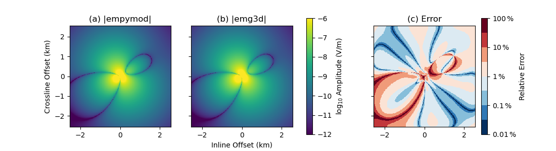
ax1.set_title(r"(a) |empymod|")
cf0 = ax1.pcolormesh(x3, x3, np.log10(epm.amp()), **a_kwargs)
ax2.set_title(r"(b) |emg3d|")
ax2.pcolormesh(x3, x3, np.log10(e3d.amp()), **a_kwargs)
ax3.set_title(r"(c) Error")
rel_error = 100*np.abs((epm - e3d) / epm)
cf2 = ax3.pcolormesh(x3, x3, np.log10(rel_error), **e_kwargs)
# Colorbars
fig.colorbar(cf0, ax=axs[:2], label=r"$\log_{10}$ Amplitude (V/m)")
cbar = fig.colorbar(cf2, ax=ax3, label=r"Relative Error")
cbar.set_ticks([-2, -1, 0, 1, 2])
cbar.ax.set_yticklabels([r"$0.01\,\%$", r"$0.1\,\%$", r"$1\,\%$",
r"$10\,\%$", r"$100\,\%$"])
ax1.set_xlim(min(x3), max(x3))
ax1.set_ylim(min(x3), max(x3))
# Axis label
ax1.set_ylabel("Crossline Offset (km)")
ax2.set_xlabel("Inline Offset (km)")
print(f"- Source: {source}")
print(f"- Frequency: {sval} Hz")
print(f"- Electric receivers: z={rz} m; θ={azimuth}°, φ={elevation}°")
- Source: TxElectricDipole: 3.1 A;
    e1={-50.0; -30.0; -320.0} m; e2={50.0; 30.0; -280.0} m
- Frequency: -7 Hz
- Electric receivers: z=-400.0 m; θ=33°, φ=18°
Total running time of the script: (0 minutes 15.265 seconds)
Estimated memory usage: 257 MB