Note
Go to the end to download the full example code.
GemPy-I: Simple Fault Model#
This example uses GemPy to create a geological model as input to emg3d, utilizing discretize. Having it in discretize allows us also to plot it with PyVista.
The starting point is the simple_fault_model as used in Chapter 1.1 of the GemPy documentation. It is a nice, made-up model of a folded structure with a fault. Here we slightly modify it (convert it into a shallow marine setting), and create a resisistivity model out of the lithological model.
The result is what is referred to in other examples as model GemPy-I, a synthetic, shallow-marine resistivity model consisting of a folded structure with a fault. It is one of a few models created to be used in other examples.
Note
The original model (simple_fault_model) hosted on cgre-aachen/gempy_data is released under the LGPL-3.0 License.
import os
import pooch
import emg3d
import matplotlib.pyplot as plt
from matplotlib.colors import LogNorm
plt.style.use('bmh')


# Adjust this path to a folder of your choice.
data_path = os.path.join('..', 'download', '')
Fetch the model#
Retrieve and load the pre-computed resistivity model.
fname = "GemPy-I.h5"
pooch.retrieve(
    'https://raw.github.com/emsig/data/2021-05-21/emg3d/models/'+fname,
    '06f522a69c94dc02ca3da0ea4ca7b60f7a9c764cdcbf6699ef4155621d70b3bb',
    fname=fname,
    path=data_path,
)
fmodel = emg3d.load(data_path + fname)['model']
fgrid = fmodel.grid
Data loaded from «/home/dtr/Codes/emsig/emg3d-gallery/examples/download/GemPy-I.h5»
[emg3d v1.0.0rc3.dev5+g0cd9e09 (format 1.0) on 2021-05-21T14:06:32.551618].
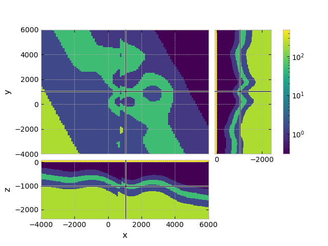
QC resistivity model#
fgrid.plot_3d_slicer(
    fmodel.property_x, zslice=-1000,
    pcolor_opts={'norm': LogNorm(vmin=0.3, vmax=500)}
)
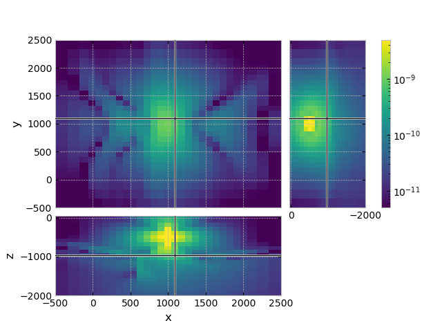
Compute some example CSEM data with it#
# Source:  x-directed electric-source at (1000, 1000, -500)
src_coo = [1000, 1000, -500, 0, 0]
frequency = 1.0  # Hz

# Computational grid
grid = emg3d.construct_mesh(
    frequency=frequency,
    center=src_coo[:3],
    properties=[0.3, 200, 1000],
    domain=([0, 2000], [0, 2000], [-2000, 0]),
    seasurface=0,
    center_on_edge=False,
)
grid

# Get the computational model
model = fmodel.interpolate_to_grid(grid)

# Compute the response
efield = emg3d.solve_source(
    model=model,
    source=emg3d.TxElectricDipole(src_coo),
    frequency=frequency,
    verb=1,
)

# Plot the response
grid.plot_3d_slicer(
    efield.fx.ravel('F'),
    view='abs', v_type='Ex',
    zslice=-1000,
    xlim=(-500, 2500), ylim=(-500, 2500), zlim=(-2000, 50),
    pcolor_opts={'norm': LogNorm(vmin=5e-12, vmax=5e-9)},
)
:: emg3d :: 7.9e-07; 2(9); 0:00:11; CONVERGED
Reproduce the model#
Note
The following sections are about how to reproduce the model. For this you
have to install gempy. The code example and the GemPy-I.h5-file
used in the gallery were created on 2021-05-21 with gempy=2.2.9 and
pandas=1.2.4.
Get and initiate the simple_fault_model#
Changes made to the original model (differences between the files simple_fault_model_*.csv and simple_fault_model_*_geophy.csv): Changed the stratigraphic unit names, and moved the model 2 km down.
Instead of reading a csv-file we could also initiate an empty instance and then add points and orientations after that by, e.g., providing numpy arrays.
import gempy as gempy
import numpy as np

# Initiate a model
geo_model = gempy.create_model('GemPy-I')

# Location of data files.
data_url = 'https://raw.githubusercontent.com/cgre-aachen/gempy_data/'
data_url += 'master/data/input_data/tut_chapter1/'

# Importing the data from CSV-files and setting extent and resolution
# This is a regular grid, mainly for plotting purposes
gempy.init_data(
    geo_model,
    [0, 2000., 0, 2000., -2000, 40.], [50, 50, 51],
    path_o=data_url+"simple_fault_model_orientations_geophy.csv",
    path_i=data_url+"simple_fault_model_points_geophy.csv",
)
Initiate the stratigraphies and faults, and add an air layer#
# Add an air-layer: Horizontal layer at z=0m
geo_model.add_surfaces('air')
geo_model.add_surface_points(0, 0, 0, 'air')
geo_model.add_surface_points(0, 0, 0, 'air')
geo_model.add_orientations(0, 0, 0, 'air', [0, 0, 1])

# Add Series for the air layer; this series will not be cut by the fault
geo_model.add_series('Air_Series')
geo_model.modify_order_series(2, 'Air_Series')
gempy.map_series_to_surfaces(geo_model, {'Air_Series': 'air'})

# Map the different series
gempy.map_series_to_surfaces(
    geo_model,
    {
        "Fault_Series": 'fault',
        "Air_Series": ('air'),
        "Strat_Series": ('seawater', 'overburden', 'target',
                         'underburden', 'basement')
    },
    remove_unused_series=True
)

geo_model.rename_series({'Main_Fault': 'Fault_Series'})

# Set which series the fault series is cutting
geo_model.set_is_fault('Fault_Series')
geo_model.faults.faults_relations_df
Compute the model with GemPy#
# Set the interpolator.
gempy.set_interpolator(
    geo_model,
    compile_theano=True,
    theano_optimizer='fast_compile',
    verbose=[]
)

# Compute it.
sol = gempy.compute_model(geo_model, compute_mesh=True)

# Plot lithologies (colour-code corresponds to lithologies)
_ = gempy.plot_2d(geo_model, cell_number=25, direction='y',
                  show_data=True)
Get id’s for a discretize mesh#
We could define the resistivities before, but currently it is difficult for
GemPy to interpolate for something like resistivities with a very wide range
of values (several orders of magnitudes). So we can simply map it here to the
id (Note: GemPy does not do interpolation for cells which lie in
different stratigraphies, so the id is always in integer).
# First we create a detailed discretize-mesh to store the resistivity
# model and use it in other examples as well.
hxy = np.ones(100)*100
hz = np.ones(100)*25
fgrid = emg3d.TensorMesh([hxy, hxy, hz], origin=(-4000, -4000, -2400))

# Get the solution at cell centers of our grid.
sol = gempy.compute_model(geo_model, at=fgrid.gridCC)

# Show the surfaces.
geo_model.surfaces
Replace id’s by resistivities#
# Now, we convert the id's to resistivities
res = sol.custom[0][0, :fgrid.n_cells]

res[res == 1] = 1e8  # air
# id=2 is the fault
res[np.round(res) == 3] = 0.3  # sea water
res[np.round(res) == 4] = 1.0  # overburden
res[np.round(res) == 5] = 50   # resistive layer
res[np.round(res) == 6] = 1.5  # underburden
res[np.round(res) == 7] = 200  # resistive basement

# Create an emg3d-model.
fmodel = emg3d.Model(fgrid, property_x=res, mapping='Resistivity')

# Store model.
emg3d.save('GemPy-I.h5', model=fmodel)
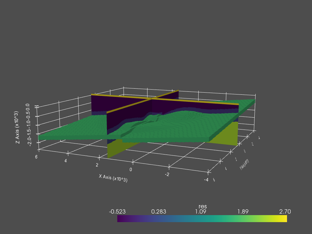
PyVista plot#
Note
The final cell is about how to plot the model in 3D using PyVista,
for which you have to install pyvista.
The code example was created on 2021-05-21 with pyvista=0.30.1.
import pyvista
import numpy as np

dataset = fgrid.toVTK({'res': np.log10(fmodel.property_x.ravel('F'))})

# Create the rendering scene and add a grid axes
p = pyvista.Plotter(notebook=True)
p.show_grid(location='outer')

# Add spatially referenced data to the scene
dparams = {'rng': np.log10([0.3, 500]), 'show_edges': False}
xyz = (1500, 500, -1500)
p.add_mesh(dataset.slice('x', xyz), name='x-slice', **dparams)
p.add_mesh(dataset.slice('y', xyz), name='y-slice', **dparams)

# Add a layer as 3D
p.add_mesh(dataset.threshold([1.69, 1.7]), name='vol', **dparams)

# Show the scene!
p.camera_position = [
    (-10000, 25000, 4000), (1000, 1000, -1000), (0, 0, 1)
]
p.show()
Total running time of the script: (0 minutes 12.508 seconds)
Estimated memory usage: 335 MB