2. MARE2DEM: 2D with tri-axial anisotropy

MARE2DEM is an open-source, finite element 2.5D code for controlled-source electromagnetic (CSEM) and magnetotelluric (MT) data, see mare2dem.bitbucket.io.

Note

The MARE2DEM results are pre-computed. All input files to reproduce the results are available on https://github.com/emsig/data/tree/main/emg3d/external/MARE2DEM .

import os
import pooch
import emg3d
import numpy as np
import matplotlib.pyplot as plt
from matplotlib.colors import LogNorm
plt.style.use('bmh')


# Adjust this path to a folder of your choice.
data_path = os.path.join('..', 'download', '')

Fetch and load MARE2DEM result

url = 'https://raw.github.com/emsig/data/2021-05-21/emg3d/external/MARE2DEM/'
fname1 = 'triaxial.0.resp'
pooch.retrieve(
    url + fname1,
    '29ec8e3dbfc615bcb430df5cbd89fea6302bb3867d90ae969907314013dc871b',
    fname=fname1,
    path=data_path,
)
mar_tg = np.loadtxt(data_path + fname1, skiprows=93, usecols=6)
mar_tg = mar_tg[::2] + 1j*mar_tg[1::2]

fname2 = 'triaxial-BG.0.resp'
pooch.retrieve(
    url + fname2,
    '036f72e30b7794304c45ef73403cdd8318ca0fc5c2fdbe7d05a33731cf3f2cf6',
    fname=fname2,
    path=data_path,
)
mar_bg = np.loadtxt(data_path + fname2, skiprows=93, usecols=6)
mar_bg = mar_bg[::2] + 1j*mar_bg[1::2]

emg3d

In order to shorten the build-time of the gallery we use a coarse model. Set coarse_model = False to obtain a result of higher accuracy.

coarse_model = True

# Source location [x, y, z, azimuth, elevation]
source = emg3d.TxElectricDipole((50, 0, -1950, 0, 0))
rec = (np.arange(80)*100+2050, 0, -1999.9, 0, 0)
frequency = 0.5             # Frequency (Hz)

if coarse_model:
    min_width = 100
    stretching = ([1.02, 1.5], [1.05, 1.5], [1, 1.5])
else:
    min_width = 50
    stretching = [1, 1.5]

# Create grid.
grid = emg3d.construct_mesh(
    frequency=frequency,
    properties=[0.3, 1, 100],
    center=(0, 0, -2000),
    domain=([-100, 10100], [-1000, 1000], [-4200, 0]),
    stretching=stretching,
    min_width_limits=min_width,
    center_on_edge=True,
)
grid

TensorMesh			245,760 cells
		MESH EXTENT		CELL WIDTH		FACTOR
dir	nC	min	max	min	max	max
x	80	-50,416.82	55,590.88	100.00	16,432.88	1.48
y	48	-46,181.63	46,181.63	100.00	13,445.46	1.42
z	64	-9,432.76	45,181.63	100.00	13,445.46	1.42

xx = (grid.cell_centers[:, 0] > 0)*(grid.cell_centers[:, 0] <= 6000)
zz = (grid.cell_centers[:, 2] > -4200)*(grid.cell_centers[:, 2] < -4000)

# Background
res_x_full = 2*np.ones(grid.n_cells)
res_y_full = 1*np.ones(grid.n_cells)
res_z_full = 3*np.ones(grid.n_cells)

# Water - isotropic
res_x_full[grid.cell_centers[:, 2] >= -2000] = 0.3
res_y_full[grid.cell_centers[:, 2] >= -2000] = 0.3
res_z_full[grid.cell_centers[:, 2] >= -2000] = 0.3

# Air - isotropic
res_x_full[grid.cell_centers[:, 2] >= 0] = 1e10
res_y_full[grid.cell_centers[:, 2] >= 0] = 1e10
res_z_full[grid.cell_centers[:, 2] >= 0] = 1e10

# Target
res_x_full_tg = res_x_full.copy()
res_y_full_tg = res_y_full.copy()
res_z_full_tg = res_z_full.copy()
res_x_full_tg[xx*zz] = 200
res_y_full_tg[xx*zz] = 100
res_z_full_tg[xx*zz] = 300

# Collect models
model_bg = emg3d.Model(
        grid, property_x=res_x_full, property_y=res_y_full,
        property_z=res_z_full, mapping='Resistivity')
model_tg = emg3d.Model(
        grid, property_x=res_x_full_tg, property_y=res_y_full_tg,
        property_z=res_z_full_tg, mapping='Resistivity')

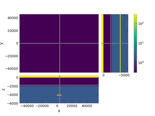
# QC model
grid.plot_3d_slicer(
        model_tg.property_x, zlim=[-6000, 500],
        pcolor_opts={'norm': LogNorm(vmin=0.3, vmax=300)})

Model background

efield_bg = emg3d.solve_source(model_bg, source, frequency)
e3d_bg = efield_bg.get_receiver(rec)

Model target

efield_tg = emg3d.solve_source(model_tg, source, frequency)
e3d_tg = efield_tg.get_receiver(rec)

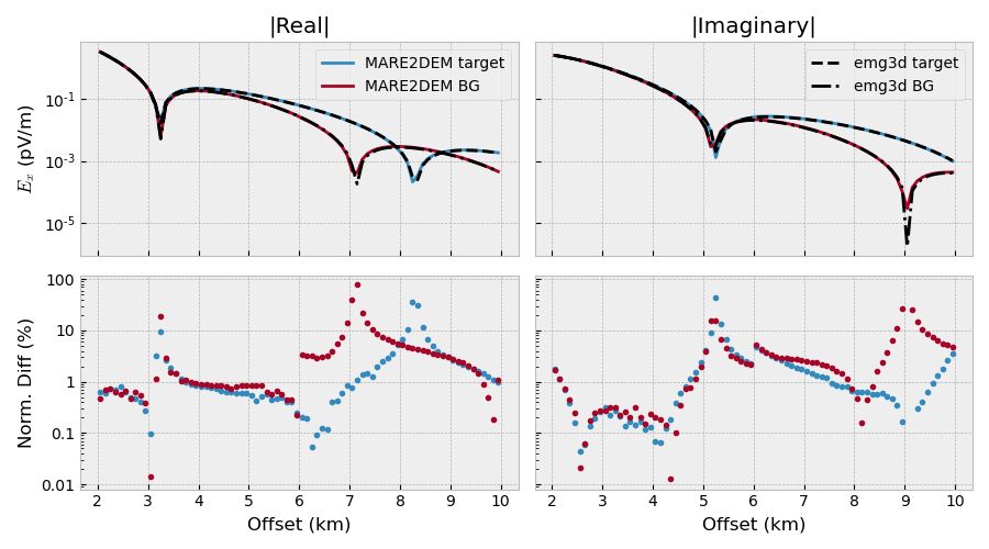
Plot

def nrmsd(a, b):
    """Return Normalized Root-Mean-Square Difference."""
    return 200 * abs(a - b) / (abs(a) + abs(b))


fig, axs = plt.subplots(2, 2, figsize=(9, 5), sharex=True, sharey='row')
((ax1, ax3), (ax2, ax4)) = axs

# Real part
ax1.set_title(r'|Real|')
ax1.plot(rec[0]/1e3, 1e12*np.abs(mar_tg.real), 'C0-', label='MARE2DEM target')
ax1.plot(rec[0]/1e3, 1e12*np.abs(mar_bg.real), 'C1-', label='MARE2DEM BG')
ax1.plot(rec[0]/1e3, 1e12*np.abs(e3d_tg.real), 'k--')
ax1.plot(rec[0]/1e3, 1e12*np.abs(e3d_bg.real), 'k-.')
ax1.set_ylabel('$E_x$ (pV/m)')
ax1.set_yscale('log')
ax1.legend()

# Normalized difference real
ax2.plot(rec[0]/1e3, nrmsd(mar_tg.real, e3d_tg.real), 'C0.')
ax2.plot(rec[0]/1e3, nrmsd(mar_bg.real, e3d_bg.real), 'C1.')
ax2.set_ylabel('Norm. Diff (%)')
ax2.set_xlabel('Offset (km)')

# Imaginary part
ax3.set_title(r'|Imaginary|')
ax3.plot(rec[0]/1e3, 1e12*np.abs(mar_tg.imag), 'C0-')
ax3.plot(rec[0]/1e3, 1e12*np.abs(mar_bg.imag), 'C1-')
ax3.plot(rec[0]/1e3, 1e12*np.abs(e3d_tg.imag), 'k--', label='emg3d target')
ax3.plot(rec[0]/1e3, 1e12*np.abs(e3d_bg.imag), 'k-.', label='emg3d BG')
ax3.legend()

# Normalized difference imag
ax4.plot(rec[0]/1e3, nrmsd(mar_tg.imag, e3d_tg.imag), 'C0.')
ax4.plot(rec[0]/1e3, nrmsd(mar_bg.imag, e3d_bg.imag), 'C1.')
ax4.set_xlabel('Offset (km)')
ax4.set_yscale('log')
ax4.set_ylim([8e-3, 120])
ax4.set_yticks([0.01, 0.1, 1, 10, 100])
ax4.set_yticklabels(('0.01', '0.1', '1', '10', '100'))

fig.tight_layout()
fig.show()

emg3d.Report()

Wed Aug 31 21:42:23 2022 CEST
OS	Linux	CPU(s)	4	Machine	x86_64
Architecture	64bit	RAM	15.5 GiB	Environment	Python
File system	ext4
Python 3.9.12 | packaged by conda-forge | (main, Mar 24 2022, 23:22:55) [GCC 10.3.0]
numpy	1.22.4	scipy	1.9.0	numba	0.55.2
emg3d	1.8.0	empymod	2.2.0	xarray	2022.6.0
discretize	0.8.2	h5py	3.7.0	matplotlib	3.4.3
tqdm	4.64.0	IPython	8.4.0
Intel(R) oneAPI Math Kernel Library Version 2022.0-Product Build 20211112 for Intel(R) 64 architecture applications

Estimated memory usage: 214 MB