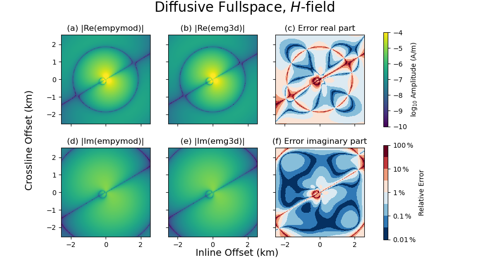
6. Magnetic field due to an el. source

The solver emg3d returns the electric field in x-, y-, and z-direction. Using Farady’s law of induction we can obtain the magnetic field from it. Faraday’s law of induction in the frequency domain can be written as, in its differential form,

(1)\[\nabla \times \mathbf{E} = \rm{i}\omega \mathbf{B} = \rm{i}\omega\mu\mathbf{H}\, .\]

This is exactly what we do in this example, for a rotated finite length bipole in a homogeneous VTI fullspace, and compare it to the semi-analytical solution of empymod. (The code empymod is an open-source code which can model CSEM responses for a layered medium including VTI electrical anisotropy, see emsig.xyz.)

import emg3d
import empymod
import numpy as np
import matplotlib.pyplot as plt

Full-space model for a finite length, finite strength, rotated bipole

In order to shorten the build-time of the gallery we use a coarse model. Set coarse_model = False to obtain a result of higher accuracy.

coarse_model = True

Survey and model parameters

# Receiver coordinates
if coarse_model:
    x = (np.arange(256))*20-2550
else:
    x = (np.arange(1025))*5-2560
rx = np.repeat([x, ], np.size(x), axis=0)
ry = rx.transpose()
frx, fry = rx.ravel(), ry.ravel()
rz = -400.0
azimuth = 30
elevation = 10

# Source coordinates, frequency, and strength
source = emg3d.TxElectricDipole(
    coordinates=[-50, 50, -30, 30, -320., -280.],  # [x1, x2, y1, y2, z1, z2]
    strength=3.3,  # A
)
frequency = 0.8  # Hz

# Model parameters
h_res = 1.              # Horizontal resistivity
aniso = np.sqrt(2.)     # Anisotropy
v_res = h_res*aniso**2  # Vertical resistivity

empymod

Note: The coordinate system of empymod is positive z down, for emg3d it is positive z up. We have to switch therefore src_z, rec_z, and elevation.

# Compute
epm = empymod.bipole(
    src=np.r_[source.coordinates[:4], -source.coordinates[4:]],
    rec=[frx, fry, -rz, azimuth, -elevation],
    depth=[],
    res=h_res,
    aniso=aniso,
    strength=source.strength,
    srcpts=5,
    freqtime=frequency,
    htarg={'pts_per_dec': -1},
    mrec=True,
    verb=3,
).reshape(np.shape(rx))

:: empymod START  ::  v2.2.0

   depth       [m] :
   res     [Ohm.m] :  1
   aniso       [-] :  1.41421
   epermH      [-] :  1
   epermV      [-] :  1
   mpermH      [-] :  1
   mpermV      [-] :  1

>  MODEL IS A FULLSPACE
   direct field    :  Comp. in wavenumber domain
   frequency  [Hz] :  0.8
   Hankel          :  DLF (Fast Hankel Transform)
     > Filter      :  Key 201 (2009)
     > DLF type    :  Lagged Convolution
   Loop over       :  Frequencies
   Source(s)       :  1 bipole(s)
     > intpts      :  5
     > length  [m] :  123.288
     > strength[A] :  3.3
     > x_c     [m] :  0
     > y_c     [m] :  0
     > z_c     [m] :  300
     > azimuth [°] :  30.9638
     > dip     [°] :  -18.9318
   Receiver(s)     :  65536 dipole(s)
     > x       [m] :  -2550 - 2550 : 65536  [min-max; #]
     > y       [m] :  -2550 - 2550 : 65536  [min-max; #]
     > z       [m] :  400
     > azimuth [°] :  30
     > dip     [°] :  -10
   Required ab's   :  14 24 34 15 25 35 16 26 36

:: empymod END; runtime = 0:00:00.671096 :: 40 kernel call(s)

emg3d

if coarse_model:
    min_width_limits = 40
    stretching = [1.045, 1.045]
else:
    min_width_limits = 20
    stretching = [1.03, 1.045]

# Create stretched grid
grid = emg3d.construct_mesh(
    frequency=frequency,
    properties=h_res,
    center=source.center,
    domain=([-2500, 2500], [-2500, 2500], [-2900, 2100]),
    min_width_limits=min_width_limits,
    stretching=stretching,
    lambda_from_center=True,
    lambda_factor=0.8,
    center_on_edge=False,
)
grid

TensorMesh			512,000 cells
		MESH EXTENT		CELL WIDTH		FACTOR
dir	nC	min	max	min	max	max
x	80	-4,155.20	4,378.72	40.00	223.51	1.04
y	80	-4,155.20	4,378.72	40.00	223.51	1.04
z	80	-4,566.91	3,752.18	40.00	214.73	1.04

# Define the model
model = emg3d.Model(
    grid, property_x=h_res, property_z=v_res, mapping='Resistivity')

# Compute the electric field
efield = emg3d.solve_source(model, source, frequency, verb=4, plain=True)

:: emg3d START :: 21:47:20 :: v1.8.0

   MG-cycle       : 'F'                 sslsolver : False
   semicoarsening : False [0]           tol       : 1e-06
   linerelaxation : False [0]           maxit     : 50
   nu_{i,1,c,2}   : 0, 2, 1, 2          verb      : 4
   Original grid  :  80 x  80 x  80     => 512,000 cells
   Coarsest grid  :   5 x   5 x   5     => 125 cells
   Coarsest level :   4 ;   4 ;   4

   [hh:mm:ss]  rel. error                  [abs. error, last/prev]   l s

       h_
      2h_ \                  /
      4h_  \          /\    /
      8h_   \    /\  /  \  /
     16h_    \/\/  \/    \/

   [21:47:23]   3.602e-02  after   1 F-cycles   [3.540e-05, 0.036]   0 0
   [21:47:25]   3.766e-03  after   2 F-cycles   [3.701e-06, 0.105]   0 0
   [21:47:28]   5.020e-04  after   3 F-cycles   [4.933e-07, 0.133]   0 0
   [21:47:30]   7.497e-05  after   4 F-cycles   [7.367e-08, 0.149]   0 0
   [21:47:33]   1.211e-05  after   5 F-cycles   [1.190e-08, 0.162]   0 0
   [21:47:35]   2.223e-06  after   6 F-cycles   [2.184e-09, 0.184]   0 0
   [21:47:38]   6.236e-07  after   7 F-cycles   [6.128e-10, 0.281]   0 0

   > CONVERGED
   > MG cycles        : 7
   > Final rel. error : 6.236e-07

:: emg3d END   :: 21:47:38 :: runtime = 0:00:18

Compute magnetic field \(H\) from the electric field

hfield = emg3d.get_magnetic_field(model, efield)

# Get responses at receivers
e3d = hfield.get_receiver((rx, ry, rz, azimuth, elevation))

Plot

# Start figure.
a_kwargs = {'cmap': "viridis", 'vmin': -10, 'vmax': -4, 'shading': 'nearest'}

e_kwargs = {'cmap': plt.cm.get_cmap("RdBu_r", 8),
            'vmin': -2, 'vmax': 2, 'shading': 'nearest'}

fig, axs = plt.subplots(2, 3, figsize=(10, 5.5), sharex=True, sharey=True,
                        subplot_kw={'box_aspect': 1})

((ax1, ax2, ax3), (ax4, ax5, ax6)) = axs
x3 = x/1000  # km

# Plot Re(data)
ax1.set_title(r"(a) |Re(empymod)|")
cf0 = ax1.pcolormesh(x3, x3, np.log10(epm.real.amp()), **a_kwargs)

ax2.set_title(r"(b) |Re(emg3d)|")
ax2.pcolormesh(x3, x3, np.log10(e3d.real.amp()), **a_kwargs)

ax3.set_title(r"(c) Error real part")
rel_error = 100*np.abs((epm.real - e3d.real) / epm.real)
cf2 = ax3.pcolormesh(x3, x3, np.log10(rel_error), **e_kwargs)

# Plot Im(data)
ax4.set_title(r"(d) |Im(empymod)|")
ax4.pcolormesh(x3, x3, np.log10(epm.imag.amp()), **a_kwargs)

ax5.set_title(r"(e) |Im(emg3d)|")
ax5.pcolormesh(x3, x3, np.log10(e3d.imag.amp()), **a_kwargs)

ax6.set_title(r"(f) Error imaginary part")
rel_error = 100*np.abs((epm.imag - e3d.imag) / epm.imag)
ax6.pcolormesh(x3, x3, np.log10(rel_error), **e_kwargs)

# Colorbars
fig.colorbar(cf0, ax=axs[0, :], label=r"$\log_{10}$ Amplitude (A/m)")
cbar = fig.colorbar(cf2, ax=axs[1, :], label=r"Relative Error")
cbar.set_ticks([-2, -1, 0, 1, 2])
cbar.ax.set_yticklabels([r"$0.01\,\%$", r"$0.1\,\%$", r"$1\,\%$",
                         r"$10\,\%$", r"$100\,\%$"])

ax1.set_xlim(min(x3), max(x3))
ax1.set_ylim(min(x3), max(x3))

# Axis label
fig.text(0.4, 0.05, "Inline Offset (km)", fontsize=14)
fig.text(0.05, 0.3, "Crossline Offset (km)", rotation=90, fontsize=14)
fig.suptitle(r'Diffusive Fullspace, $H$-field', y=1, fontsize=20)

print(f"- Source: {source}")
print(f"- Frequency: {frequency} Hz")
print(f"- Magnetic receivers: z={rz} m; θ={azimuth}°, φ={elevation}°")

fig.show()

- Source: TxElectricDipole: 3.3 A;
    e1={-50.0; -30.0; -320.0} m; e2={50.0; 30.0; -280.0} m
- Frequency: 0.8 Hz
- Magnetic receivers: z=-400.0 m; θ=30°, φ=10°

emg3d.Report()

Wed Aug 31 21:47:40 2022 CEST
OS	Linux	CPU(s)	4	Machine	x86_64
Architecture	64bit	RAM	15.5 GiB	Environment	Python
File system	ext4
Python 3.9.12 | packaged by conda-forge | (main, Mar 24 2022, 23:22:55) [GCC 10.3.0]
numpy	1.22.4	scipy	1.9.0	numba	0.55.2
emg3d	1.8.0	empymod	2.2.0	xarray	2022.6.0
discretize	0.8.2	h5py	3.7.0	matplotlib	3.4.3
tqdm	4.64.0	IPython	8.4.0
Intel(R) oneAPI Math Kernel Library Version 2022.0-Product Build 20211112 for Intel(R) 64 architecture applications

Estimated memory usage: 112 MB