Note
Go to the end to download the full example code.
03. Simulation#
The easiest way to model CSEM data for a survey is to make use of the Survey
and Simulation classes, emg3d.surveys.Survey and
emg3d.simulations.Simulation, respectively, together with the
automatic gridding functionality.
For this example we use the resistivity model created in the example GemPy-II: Perth Basin.
import os
import pooch
import emg3d
import numpy as np
import matplotlib.pyplot as plt
from matplotlib.colors import LogNorm
from scipy.interpolate import RectBivariateSpline
plt.style.use('bmh')


# Adjust this path to a folder of your choice.
data_path = os.path.join('..', 'download', '')
Fetch the model#
Retrieve and load the pre-computed resistivity model.
fname = "GemPy-II.h5"
pooch.retrieve(
    'https://raw.github.com/emsig/data/2021-05-21/emg3d/models/'+fname,
    'ea8c23be80522d3ca8f36742c93758370df89188816f50cb4e1b2a6a3012d659',
    fname=fname,
    path=data_path,
)
model = emg3d.load(data_path + fname)['model']
Data loaded from «/home/dtr/Codes/emsig/emg3d-gallery/examples/download/GemPy-II.h5»
[emg3d v1.0.0rc3.dev5+g0cd9e09 (format 1.0) on 2021-05-21T18:40:16.721968].
Let’s check the model
So it is an isotropic model defined in terms of resistivities. Let’s check the grid
Define the survey#
If you have actual field data then this info would normally come from a data file or similar. Here we create our own dummy survey, and later will create synthetic data for it.
A Survey instance contains all survey-related information, hence source
and receiver positions and measured data. See the relevant documentation for
more details: emg3d.surveys.Survey.
Extract seafloor to simulate source and receiver depths#
To create a realistic survey we create a small routine that finds the seafloor, so we can place receivers on the seafloor and sources 50 m above it. We use the fact that the seawater has resistivity of 0.3 Ohm.m in the model, and is the lowest value.
seafloor = np.ones((grid.shape_cells[0], grid.shape_cells[1]))
for i in range(grid.shape_cells[0]):
    for ii in range(grid.shape_cells[1]):
        # We take the seafloor to be the first cell which resistivity
        # is below 0.33
        seafloor[i, ii] = grid.nodes_z[:-1][
                model.property_x[i, ii, :] < 0.33][0]

# Create a 2D interpolation function from it
bathymetry = RectBivariateSpline(
        grid.cell_centers_x, grid.cell_centers_y, seafloor)
Source and receiver positions#
Sources and receivers can be defined in a few different ways. One way is by providing coordinates, where two coordinate formats are accepted:
(x0, x1, y0, y1, z0, z1): finite length dipole,(x, y, z, azimuth, elevation): point dipole,
where the angles (azimuth and elevation) are in degrees. For the coordinate system see coordinate_system.
A survey can contain electric and magnetic receivers, arbitrarily rotated.
However, the Simulation is currently limited to electric receivers.
Note that the survey just knows about the sources, receivers, frequencies, and observed data - it does not know anything of an underlying model.
# Angles for horizontal, x-directed Ex point dipoles
elevation = 0.0
azimuth = 0.0

# Acquisition source frequencies (Hz)
frequencies = [0.5, 1.0]

# Source coordinates
src_x = np.arange(1, 4)*5000
src_y = 7500
# Source depths: 50 m above seafloor
src_z = bathymetry(src_x, src_y).ravel()+50
src = emg3d.surveys.txrx_coordinates_to_dict(
        emg3d.TxElectricDipole,
        (src_x, src_y, src_z, azimuth, elevation)
)

# Receiver positions
rec_x = np.arange(3, 18)*1e3
rec_y = np.arange(3)*1e3+6500
RX, RY = np.meshgrid(rec_x, rec_y, indexing='ij')
RZ = bathymetry(rec_x, rec_y)
rec = emg3d.surveys.txrx_coordinates_to_dict(
        emg3d.RxElectricPoint,
        (RX.ravel(), RY.ravel(), RZ.ravel(), azimuth, elevation)
)
Create Survey#
If you have observed data you can provide them, here we will create synthetic
data later on. What you have to define is the expected noise floor and
relative error, which is used to compute the misfit later on. Alternatively
you can provide directly the standard deviation; see
emg3d.surveys.Survey.
survey = emg3d.surveys.Survey(
    name='GemPy-II Survey A',  # Name of the survey
    sources=src,               # Source coordinates
    receivers=rec,             # Receiver coordinates
    frequencies=frequencies,   # Two frequencies
    # data=data,               # If you have observed data
    noise_floor=1e-15,
    relative_error=0.05,
)

# Let's have a look at the survey:
survey
Our survey has our sources and receivers and initiated a variable
observed, with NaN’s. Each source and receiver got a name assigned. If
you prefer other names you would have to define the sources and receivers
through emg3d.surveys.Dipole, and provide a list of dipoles to the survey
instead of only a tuple of coordinates.
We can also look at a particular source or receiver, e.g.,
survey.sources['TxED-1']
Which shows you all you need to know about a particular dipole: name, type (electric or magnetic), coordinates of its center, angles, and length.
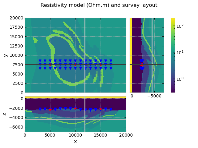
QC model and survey#
grid.plot_3d_slicer(model.property_x, xslice=12000, yslice=7500,
                    pcolor_opts={'norm': LogNorm(vmin=0.3, vmax=200)})

# Plot survey in figure above
fig = plt.gcf()
fig.suptitle('Resistivity model (Ohm.m) and survey layout')
axs = fig.get_children()
rec_coords = survey.receiver_coordinates()
src_coords = survey.source_coordinates()
axs[1].plot(rec_coords[0], rec_coords[1], 'bv')
axs[2].plot(rec_coords[0], rec_coords[2], 'bv')
axs[3].plot(rec_coords[2], rec_coords[1], 'bv')
axs[1].plot(src_coords[0], src_coords[1], 'r*')
axs[2].plot(src_coords[0], src_coords[2], 'r*')
axs[3].plot(src_coords[2], src_coords[1], 'r*')
Create a Simulation (to compute ‘observed’ data)#
The simulation class combines a model with a survey, and can compute synthetic data for it.
Automatic gridding#
We use the automatic gridding feature implemented in the simulation class to use source- and frequency- dependent grids for the computation. Consult the following docs for more information:
gridding_opts in
emg3d.simulations.Simulation;
gopts = {
    'properties': [0.3, 10, 1., 0.3],
    'min_width_limits': (100, 100, 50),
    'stretching': (None, None, [1.05, 1.5]),
    'domain': (
        [rec_coords[0].min()-100, rec_coords[0].max()+100],
        [rec_coords[1].min()-100, rec_coords[1].max()+100],
        [-5500, -2000]
    ),
    'center_on_edge': False,
}
Now we can initiate the simulation class and QC it:
simulation = emg3d.simulations.Simulation(
    name="True Model",    # A name for this simulation
    survey=survey,        # Our survey instance
    model=model,          # The model
    gridding='both',      # Frequency- and source-dependent meshes
    max_workers=4,        # How many parallel jobs
    # solver_opts,        # Any parameter to pass to emg3d.solve
    gridding_opts=gopts,  # Gridding options
)

# Let's QC our Simulation instance
simulation
Compute the data#
We pass here the argument observed=True; this way, the synthetic data is
stored in our Survey as observed data, otherwise it would be stored as
synthetic. This is important later for optimization. It also adds
Gaussian noise according to the noise floor and relative error we defined in
the survey. By setting a minimum offset the receivers close to the source are
switched off.
This computes all results in parallel; in this case six models, three sources
times two frequencies. You can change the number of workers at any time by
setting simulation.max_workers.
simulation.compute(observed=True, min_offset=500)
Compute efields            0/6  [00:00]
Compute efields █▋         1/6  [00:25]
Compute efields ████████▎  5/6  [00:41]
Compute efields ██████████ 6/6  [00:41]
A Simulation has a few convenience functions, e.g.:
simulation.get_efield('TxED-1', 0.5): Returns the electric field of the entire domain for source'TxED-1'and frequency 0.5 Hz.simulation.get_hfield;simulation.get_sfield: Similar functions to retrieve the magnetic fields and the source fields.simulation.get_model;simulation.get_grid: Similar functions to retrieve the computational grid and the model for a given source and frequency.
When we now look at our survey we see that the observed data variable is
filled with the responses at the receiver locations. Note that the
synthetic data is the actual computed data, the observed data, on the
other hand, has Gaussian noise added and is set to NaN’s for positions too
close to the source.
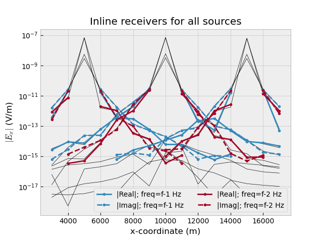
QC Data#
plt.figure()
plt.title("Inline receivers for all sources")
obs = simulation.data.observed[:, 1::3, :]
syn = simulation.data.synthetic[:, 1::3, :]
for i, src in enumerate(survey.sources.keys()):
    for ii, freq in enumerate(survey.frequencies):
        plt.plot(rec_coords[0][1::3],
                 abs(syn.loc[src, :, freq].data.real),
                 "k-", lw=0.5)
        plt.plot(rec_coords[0][1::3],
                 abs(syn.loc[src, :, freq].data.imag),
                 "k-", lw=0.5)
        plt.plot(rec_coords[0][1::3],
                 abs(obs.loc[src, :, freq].data.real),
                 f"C{ii}.-",
                 label=f"|Real|; freq={freq} Hz" if i == 0 else None
                 )
        plt.plot(rec_coords[0][1::3],
                 abs(obs.loc[src, :, freq].data.imag),
                 f"C{ii}.--",
                 label=f"|Imag|; freq={freq} Hz" if i == 0 else None
                 )

plt.yscale('log')
plt.legend(ncol=2, framealpha=1)
plt.xlabel('x-coordinate (m)')
plt.ylabel('$|E_x|$ (V/m)')
How to store surveys and simulations to disk#
Survey and Simulations can store (and load) themselves to (from) disk.
A survey stores all sources, receivers, frequencies, and the observed data.
A simulation stores the survey, the model, the synthetic data. (It can also store much more, such as all electric fields, source and frequency dependent meshes and models, etc. What it actually stores is defined by the parameter
what).
# Survey file name
# survey_fname = 'GemPy-II-survey-A.h5'

# To store, run
# survey.to_file(survey_fname)  # .h5, .json, or .npz

# To load, run
# survey = emg3d.surveys.Survey.from_file(survey_fname)

# In the same manner you could store and load the entire simulation:

# Simulation file name
# simulation_fname = file-name.ending  # for ending in [h5, json, npz]

# To store, run
# simulation.to_file(simulation_fname, what='results')

# To load, run
# simulation = emg3d.simulations.Simulation.from_file(simulation_fname)
Total running time of the script: (0 minutes 44.630 seconds)
Estimated memory usage: 431 MB